ICTC 3104.3 Data Analytics and Big DataData Import and Data Wrangling with R2020-08-201 / 66

Outline

Basics of R Programming ✅
Data Import ⚙️
Data Wrangling
Data Visualization

2 / 66

Data Import

700px

3 / 66

Setup

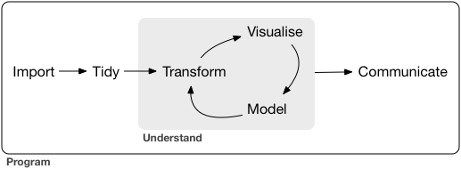install.packages("tidyverse") # install tidyverse packages
library(tidyverse) # load tidyverse packages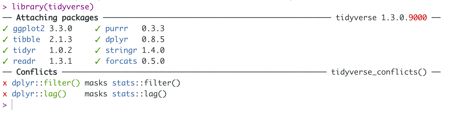

4 / 66

Tibble

Tibbles are data frames.
A modern re-imagining of data frames.

Create a tibble

library(tidyverse) # library(tibble)
first.tbl <- tibble(height = c(150, 200, 160), weight = c(45, 60, 51))
first.tbl

# A tibble: 3 x 2
  height weight
   <dbl>  <dbl>
1    150     45
2    200     60
3    160     51

class(first.tbl)

[1] "tbl_df"     "tbl"        "data.frame"

5 / 66

tibble vs. data.frame

Output

tibble

first.tbl <- tibble(height = c(150, 200, 160), weight = c(45, 60, 51))
first.tbl

# A tibble: 3 x 2
  height weight
   <dbl>  <dbl>
1    150     45
2    200     60
3    160     51

data.frame

dataframe <- data.frame(height = c(150, 200, 160), weight = c(45, 60, 51))
dataframe

  height weight
1    150     45
2    200     60
3    160     51

6 / 66

tibble vs. data.frame (cont.)

You can create new variables that are functions of existing variables.

tibble

first.tbl <- tibble(height = c(150, 200, 160), weight = c(45, 60, 51), 
                    bmi = (weight)/height^2)
first.tbl

# A tibble: 3 x 3
  height weight     bmi
   <dbl>  <dbl>   <dbl>
1    150     45 0.002  
2    200     60 0.0015 
3    160     51 0.00199

data.frame

df <- data.frame(height = c(150, 200, 160), weight = c(45, 60, 51), 
                    bmi = (weight)/height^2) # Not working

You will get an error message

Error in data.frame(height = c(150, 200, 160), weight = c(45, 60, 51), : object 'height' not found.

7 / 66

Pipe operator: %>%

Required package: `magrittr`

install.packages("magrittr")
library(magrittr)

What does it do?

It takes whatever is on the left-hand-side of the pipe and makes it the first argument of whatever function is on the right-hand-side of the pipe.

For instance,

mean(1:10)

[1] 5.5

can be written as

1:10 %>% mean()

[1] 5.5

8 / 66

🛠 Import data from a .csv file

datasetname <- read_csv("include_file_path")

When you run read_csv, it prints out the names and type of each column.

Demo: Switch to R

🛠 Importing csv file from a website

Syntax

datasetname <- read_csv("include url here")

Example

url <- "https://thiyanga.netlify.app/project/datasets/foodlabel.csv"
foodlabel <- read_csv(url)

head(foodlabel, 1)

9 / 66

🛠 Writing to a File

We can save tibble (or dataframe) to a csv file, using write_csv().
write_csv() is in the readr package.

Syntax

write_csv(name_of_the_data_set_you_want_to_save, "path_to_write_to")

Example

data(gapminder)
# This will save inside your project folder
write_csv(gaominder, "gapminder.csv") 
# This will save inside the data folder which is inside your project folder
write_csv(gapminder, "data/gapminder.csv")

Demo: Switch to R

10 / 66

🛠 Importing Excel .xlsx files

Syntax

library(readxl)
mydata <- read_xlsx("file_path")

Demo: Switch to R

11 / 66

Outline

Basics of R Programming ✅
Data Import ✅
Data Wrangling ⚙️
Data Visualization

12 / 66

Data Wrangling

700px

13 / 66

Data Wrangling/ Data Munging

14 / 66

Data Wrangling/ Data Munging

Reshaping Data (tidying your data)

How to reshape your data in order to make the analysis easier.

14 / 66

Tidy 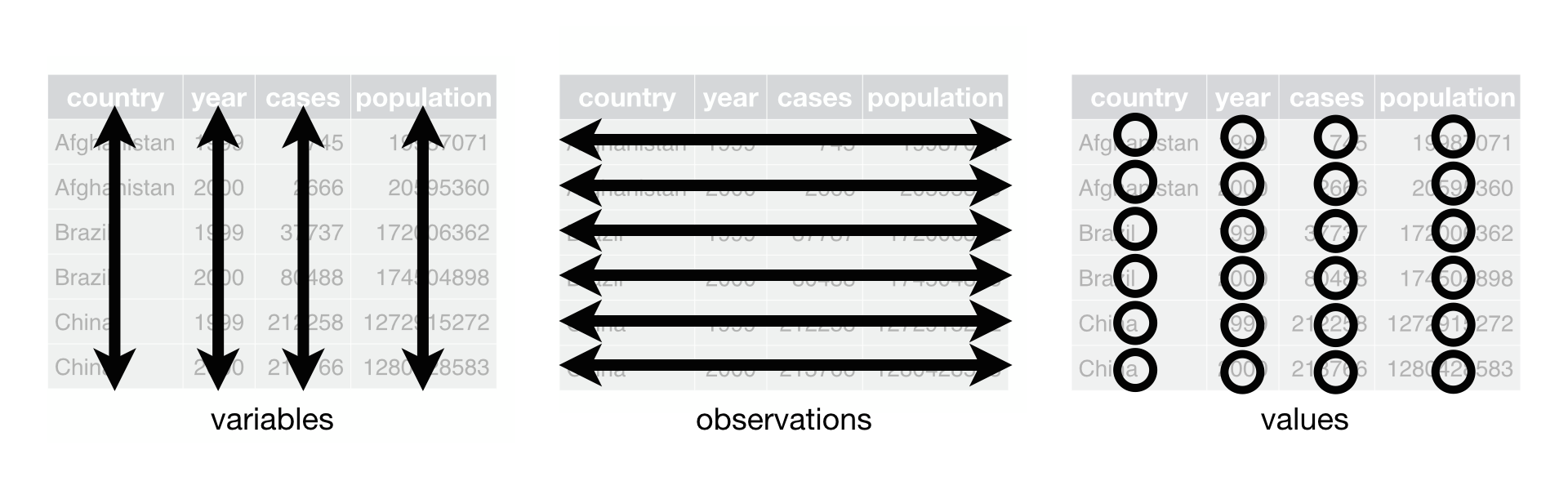Data

Figure 1: Components of a dataframe.

Each variable is saved in its column.
Each observation is saved in its own row.

Image Credit: Hadley Wickham and Garrett Grolemund

15 / 66

packages

library(tidyverse) #or library(tidyr)
library(magrittr)
library(gapminder)

16 / 66

`tidyr` package

Hadley Wickham (Chief Scientist at RStudio) is explaining tidyr at WOMBAT organized by Monash University, Australia.

knitrhex

Image rights: Thiyanga S Talagala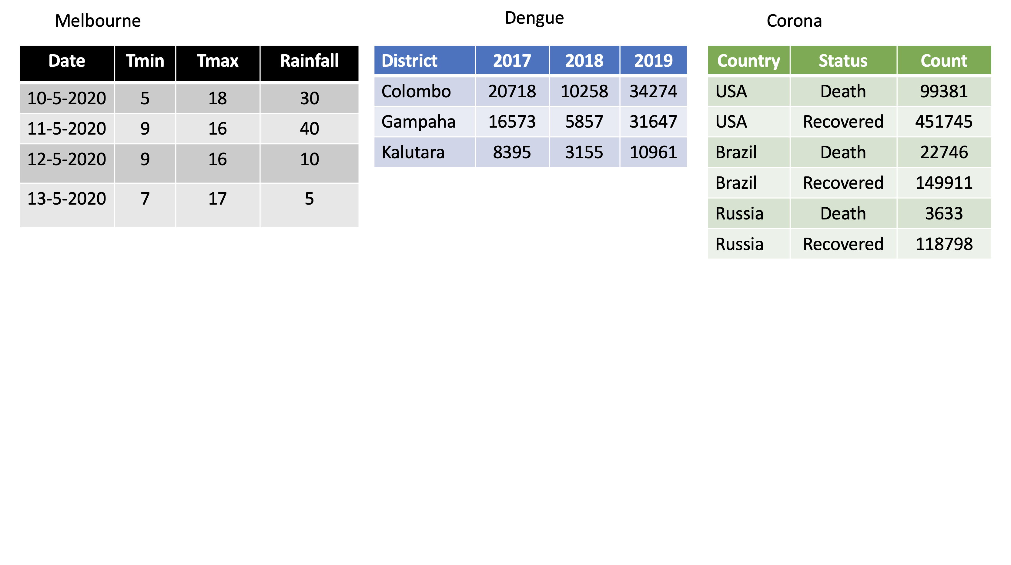

17 / 66

18 / 66

19 / 66

20 / 66

21 / 66

22 / 66

tidyr verbs

Main verbs

pivot_longer

In tidyr (2014) gather
pivot_wider

In tidyr (2014) spread

Other

separate
unite

Input and Output

Main input: data frame or tibble.

Output: tibble

23 / 66

pivot_longer24 / 66

`pivot_longer()`

Turns columns into rows.
From wide format to long format.

25 / 66

`pivot_longer()`

dengue <- tibble( dist = c("Colombo", "Gampaha", "Kalutara"), 
                  '2017' = c(20718, 10258, 34274), 
                  '2018' = c(16573, 5857, 31647), 
                  '2019' = c(8395, 3155, 10961)); dengue

# A tibble: 3 x 4
  dist     `2017` `2018` `2019`
  <chr>     <dbl>  <dbl>  <dbl>
1 Colombo   20718  16573   8395
2 Gampaha   10258   5857   3155
3 Kalutara  34274  31647  10961

dengue %>% 
  pivot_longer(2:4, names_to="Year", values_to = "Dengue counts")

# A tibble: 9 x 3
  dist     Year  `Dengue counts`
  <chr>    <chr>           <dbl>
1 Colombo  2017            20718
2 Colombo  2018            16573
3 Colombo  2019             8395
4 Gampaha  2017            10258
5 Gampaha  2018             5857
6 Gampaha  2019             3155
7 Kalutara 2017            34274
8 Kalutara 2018            31647
9 Kalutara 2019            10961

26 / 66

pivot_wider27 / 66

`pivot_wider()`

From long to wide format.

28 / 66

`pivot_wider()`

Corona <- tibble(
country = rep(c("USA", "Brazil", "Russia"), each=2),
status = rep(c("Death", "Recovered"), 3),
count = c(99381, 451745, 22746, 149911, 3633, 118798))

Corona

# A tibble: 6 x 3
  country status     count
  <chr>   <chr>      <dbl>
1 USA     Death      99381
2 USA     Recovered 451745
3 Brazil  Death      22746
4 Brazil  Recovered 149911
5 Russia  Death       3633
6 Russia  Recovered 118798

29 / 66

pivot_wider()Corona

# A tibble: 6 x 3
  country status     count
  <chr>   <chr>      <dbl>
1 USA     Death      99381
2 USA     Recovered 451745
3 Brazil  Death      22746
4 Brazil  Recovered 149911
5 Russia  Death       3633
6 Russia  Recovered 118798
Corona %>% 
  pivot_wider(names_from=status, 
              values_from=count)

# A tibble: 3 x 3
  country Death Recovered
  <chr>   <dbl>     <dbl>
1 USA     99381    451745
2 Brazil  22746    149911
3 Russia   3633    118798
30 / 66

Assign a name:

corona_wide_format <- Corona %>% 
  pivot_wider(names_from=status, 
  values_from=count)
corona_wide_format

# A tibble: 3 x 3
  country Death Recovered
  <chr>   <dbl>     <dbl>
1 USA     99381    451745
2 Brazil  22746    149911
3 Russia   3633    118798

31 / 66

`pivot_longer` vs `pivot_wider`

32 / 66

`pivot_longer` and `pivot_wider`

profit <- tibble(
year = c(2015, 2015, 2015, 2015, 2016, 2016, 2016),
quarter = c( 1, 2, 3, 4, 2, 3, 4),
income = c(2, NA, 3, NA, 4, 5, 6)
)
profit

# A tibble: 7 x 3
   year quarter income
  <dbl>   <dbl>  <dbl>
1  2015       1      2
2  2015       2     NA
3  2015       3      3
4  2015       4     NA
5  2016       2      4
6  2016       3      5
7  2016       4      6

33 / 66

`pivot_longer` and `pivot_wider`

# A tibble: 7 x 3
   year quarter income
  <dbl>   <dbl>  <dbl>
1  2015       1      2
2  2015       2     NA
3  2015       3      3
4  2015       4     NA
5  2016       2      4
6  2016       3      5
7  2016       4      6

profit %>%
pivot_wider(names_from = year, values_from = income)

# A tibble: 4 x 3
  quarter `2015` `2016`
    <dbl>  <dbl>  <dbl>
1       1      2     NA
2       2     NA      4
3       3      3      5
4       4     NA      6

34 / 66

Missing values

# A tibble: 4 x 3
  quarter `2015` `2016`
    <dbl>  <dbl>  <dbl>
1       1      2     NA
2       2     NA      4
3       3      3      5
4       4     NA      6

profit %>%
pivot_wider(names_from = year, values_from = income) %>%
pivot_longer(
cols = c(`2015`, `2016`),
names_to = "year",
values_to = "income",
values_drop_na = TRUE
)

# A tibble: 5 x 3
  quarter year  income
    <dbl> <chr>  <dbl>
1       1 2015       2
2       2 2016       4
3       3 2015       3
4       3 2016       5
5       4 2016       6

35 / 66

`dplyr` verbs

filter
select
mutate
summarise
arrange
group_by
rename

36 / 66

`filter`

Picks observations by their values.
Takes logical expressions and returns the rows for which all are TRUE.

filter(gapminder, lifeExp < 50)

# A tibble: 491 x 6
   country     continent  year lifeExp      pop gdpPercap
   <fct>       <fct>     <int>   <dbl>    <int>     <dbl>
 1 Afghanistan Asia       1952    28.8  8425333      779.
 2 Afghanistan Asia       1957    30.3  9240934      821.
 3 Afghanistan Asia       1962    32.0 10267083      853.
 4 Afghanistan Asia       1967    34.0 11537966      836.
 5 Afghanistan Asia       1972    36.1 13079460      740.
 6 Afghanistan Asia       1977    38.4 14880372      786.
 7 Afghanistan Asia       1982    39.9 12881816      978.
 8 Afghanistan Asia       1987    40.8 13867957      852.
 9 Afghanistan Asia       1992    41.7 16317921      649.
10 Afghanistan Asia       1997    41.8 22227415      635.
# … with 481 more rows

37 / 66

`filter` (cont)

filter(gapminder, country == "Sri Lanka")

# A tibble: 12 x 6
   country   continent  year lifeExp      pop gdpPercap
   <fct>     <fct>     <int>   <dbl>    <int>     <dbl>
 1 Sri Lanka Asia       1952    57.6  7982342     1084.
 2 Sri Lanka Asia       1957    61.5  9128546     1073.
 3 Sri Lanka Asia       1962    62.2 10421936     1074.
 4 Sri Lanka Asia       1967    64.3 11737396     1136.
 5 Sri Lanka Asia       1972    65.0 13016733     1213.
 6 Sri Lanka Asia       1977    65.9 14116836     1349.
 7 Sri Lanka Asia       1982    68.8 15410151     1648.
 8 Sri Lanka Asia       1987    69.0 16495304     1877.
 9 Sri Lanka Asia       1992    70.4 17587060     2154.
10 Sri Lanka Asia       1997    70.5 18698655     2664.
11 Sri Lanka Asia       2002    70.8 19576783     3015.
12 Sri Lanka Asia       2007    72.4 20378239     3970.

# gapminder %>% filter(country == "Sri Lanka")

38 / 66

`filter` (cont)

filter(gapminder, country %in% c("Sri Lanka", "Australia"))

# A tibble: 24 x 6
   country   continent  year lifeExp      pop gdpPercap
   <fct>     <fct>     <int>   <dbl>    <int>     <dbl>
 1 Australia Oceania    1952    69.1  8691212    10040.
 2 Australia Oceania    1957    70.3  9712569    10950.
 3 Australia Oceania    1962    70.9 10794968    12217.
 4 Australia Oceania    1967    71.1 11872264    14526.
 5 Australia Oceania    1972    71.9 13177000    16789.
 6 Australia Oceania    1977    73.5 14074100    18334.
 7 Australia Oceania    1982    74.7 15184200    19477.
 8 Australia Oceania    1987    76.3 16257249    21889.
 9 Australia Oceania    1992    77.6 17481977    23425.
10 Australia Oceania    1997    78.8 18565243    26998.
# … with 14 more rows

39 / 66

`filter` (cont)

filter(gapminder, country %in% c("Sri Lanka", "Australia")) %>%
  head()

# A tibble: 6 x 6
  country   continent  year lifeExp      pop gdpPercap
  <fct>     <fct>     <int>   <dbl>    <int>     <dbl>
1 Australia Oceania    1952    69.1  8691212    10040.
2 Australia Oceania    1957    70.3  9712569    10950.
3 Australia Oceania    1962    70.9 10794968    12217.
4 Australia Oceania    1967    71.1 11872264    14526.
5 Australia Oceania    1972    71.9 13177000    16789.
6 Australia Oceania    1977    73.5 14074100    18334.

filter(gapminder, country %in% c("Sri Lanka", "Australia")) %>%
  tail()

# A tibble: 6 x 6
  country   continent  year lifeExp      pop gdpPercap
  <fct>     <fct>     <int>   <dbl>    <int>     <dbl>
1 Sri Lanka Asia       1982    68.8 15410151     1648.
2 Sri Lanka Asia       1987    69.0 16495304     1877.
3 Sri Lanka Asia       1992    70.4 17587060     2154.
4 Sri Lanka Asia       1997    70.5 18698655     2664.
5 Sri Lanka Asia       2002    70.8 19576783     3015.
6 Sri Lanka Asia       2007    72.4 20378239     3970.

40 / 66

`select`

Picks variables by their names.

head(gapminder, 3)

# A tibble: 3 x 6
  country     continent  year lifeExp      pop gdpPercap
  <fct>       <fct>     <int>   <dbl>    <int>     <dbl>
1 Afghanistan Asia       1952    28.8  8425333      779.
2 Afghanistan Asia       1957    30.3  9240934      821.
3 Afghanistan Asia       1962    32.0 10267083      853.

select(gapminder, year:gdpPercap)

# A tibble: 1,704 x 4
    year lifeExp      pop gdpPercap
   <int>   <dbl>    <int>     <dbl>
 1  1952    28.8  8425333      779.
 2  1957    30.3  9240934      821.
 3  1962    32.0 10267083      853.
 4  1967    34.0 11537966      836.
 5  1972    36.1 13079460      740.
 6  1977    38.4 14880372      786.
 7  1982    39.9 12881816      978.
 8  1987    40.8 13867957      852.
 9  1992    41.7 16317921      649.
10  1997    41.8 22227415      635.
# … with 1,694 more rows

41 / 66

`select` (cont.)

head(gapminder, 3)

# A tibble: 3 x 6
  country     continent  year lifeExp      pop gdpPercap
  <fct>       <fct>     <int>   <dbl>    <int>     <dbl>
1 Afghanistan Asia       1952    28.8  8425333      779.
2 Afghanistan Asia       1957    30.3  9240934      821.
3 Afghanistan Asia       1962    32.0 10267083      853.

select(gapminder, year, gdpPercap)

# A tibble: 1,704 x 2
    year gdpPercap
   <int>     <dbl>
 1  1952      779.
 2  1957      821.
 3  1962      853.
 4  1967      836.
 5  1972      740.
 6  1977      786.
 7  1982      978.
 8  1987      852.
 9  1992      649.
10  1997      635.
# … with 1,694 more rows

42 / 66

`select` (cont.)

head(gapminder, 3)

# A tibble: 3 x 6
  country     continent  year lifeExp      pop gdpPercap
  <fct>       <fct>     <int>   <dbl>    <int>     <dbl>
1 Afghanistan Asia       1952    28.8  8425333      779.
2 Afghanistan Asia       1957    30.3  9240934      821.
3 Afghanistan Asia       1962    32.0 10267083      853.

select(gapminder, -c(year, gdpPercap))

# A tibble: 1,704 x 4
   country     continent lifeExp      pop
   <fct>       <fct>       <dbl>    <int>
 1 Afghanistan Asia         28.8  8425333
 2 Afghanistan Asia         30.3  9240934
 3 Afghanistan Asia         32.0 10267083
 4 Afghanistan Asia         34.0 11537966
 5 Afghanistan Asia         36.1 13079460
 6 Afghanistan Asia         38.4 14880372
 7 Afghanistan Asia         39.9 12881816
 8 Afghanistan Asia         40.8 13867957
 9 Afghanistan Asia         41.7 16317921
10 Afghanistan Asia         41.8 22227415
# … with 1,694 more rows

43 / 66

`select` (cont.)

head(gapminder, 3)

# A tibble: 3 x 6
  country     continent  year lifeExp      pop gdpPercap
  <fct>       <fct>     <int>   <dbl>    <int>     <dbl>
1 Afghanistan Asia       1952    28.8  8425333      779.
2 Afghanistan Asia       1957    30.3  9240934      821.
3 Afghanistan Asia       1962    32.0 10267083      853.

select(gapminder, -(year:gdpPercap))

# A tibble: 1,704 x 2
   country     continent
   <fct>       <fct>    
 1 Afghanistan Asia     
 2 Afghanistan Asia     
 3 Afghanistan Asia     
 4 Afghanistan Asia     
 5 Afghanistan Asia     
 6 Afghanistan Asia     
 7 Afghanistan Asia     
 8 Afghanistan Asia     
 9 Afghanistan Asia     
10 Afghanistan Asia     
# … with 1,694 more rows

44 / 66

`mutate`

Creates new variables with functions of existing variables

gapminder %>%
mutate(gdp = pop * gdpPercap)

# A tibble: 1,704 x 7
   country     continent  year lifeExp      pop gdpPercap          gdp
   <fct>       <fct>     <int>   <dbl>    <int>     <dbl>        <dbl>
 1 Afghanistan Asia       1952    28.8  8425333      779.  6567086330.
 2 Afghanistan Asia       1957    30.3  9240934      821.  7585448670.
 3 Afghanistan Asia       1962    32.0 10267083      853.  8758855797.
 4 Afghanistan Asia       1967    34.0 11537966      836.  9648014150.
 5 Afghanistan Asia       1972    36.1 13079460      740.  9678553274.
 6 Afghanistan Asia       1977    38.4 14880372      786. 11697659231.
 7 Afghanistan Asia       1982    39.9 12881816      978. 12598563401.
 8 Afghanistan Asia       1987    40.8 13867957      852. 11820990309.
 9 Afghanistan Asia       1992    41.7 16317921      649. 10595901589.
10 Afghanistan Asia       1997    41.8 22227415      635. 14121995875.
# … with 1,694 more rows

45 / 66

`summarise`(British) or `summarize` (US)

Collapse many values down to a single summary

gapminder %>%
  summarise(
    lifeExp_mean=mean(lifeExp),
    pop_mean=mean(pop),
    gdpPercap_mean=mean(gdpPercap))

# A tibble: 1 x 3
  lifeExp_mean  pop_mean gdpPercap_mean
         <dbl>     <dbl>          <dbl>
1         59.5 29601212.          7215.

46 / 66

`arrange`

Reorder the rows

arrange(gapminder, desc(lifeExp))

# A tibble: 1,704 x 6
   country          continent  year lifeExp       pop gdpPercap
   <fct>            <fct>     <int>   <dbl>     <int>     <dbl>
 1 Japan            Asia       2007    82.6 127467972    31656.
 2 Hong Kong, China Asia       2007    82.2   6980412    39725.
 3 Japan            Asia       2002    82   127065841    28605.
 4 Iceland          Europe     2007    81.8    301931    36181.
 5 Switzerland      Europe     2007    81.7   7554661    37506.
 6 Hong Kong, China Asia       2002    81.5   6762476    30209.
 7 Australia        Oceania    2007    81.2  20434176    34435.
 8 Spain            Europe     2007    80.9  40448191    28821.
 9 Sweden           Europe     2007    80.9   9031088    33860.
10 Israel           Asia       2007    80.7   6426679    25523.
# … with 1,694 more rows

47 / 66

`group_by`

Takes an existing tibble and converts it into a grouped tibble where operations are performed "by group". ungroup() removes grouping.

Japan_SL <- filter(gapminder, country %in% c("Japan", "Sri Lanka"))
Japan_SL %>% head()

# A tibble: 6 x 6
  country continent  year lifeExp       pop gdpPercap
  <fct>   <fct>     <int>   <dbl>     <int>     <dbl>
1 Japan   Asia       1952    63.0  86459025     3217.
2 Japan   Asia       1957    65.5  91563009     4318.
3 Japan   Asia       1962    68.7  95831757     6577.
4 Japan   Asia       1967    71.4 100825279     9848.
5 Japan   Asia       1972    73.4 107188273    14779.
6 Japan   Asia       1977    75.4 113872473    16610.

Japan_SL_grouped <- Japan_SL %>% group_by(country)
Japan_SL_grouped

# A tibble: 24 x 6
# Groups:   country [2]
   country continent  year lifeExp       pop gdpPercap
   <fct>   <fct>     <int>   <dbl>     <int>     <dbl>
 1 Japan   Asia       1952    63.0  86459025     3217.
 2 Japan   Asia       1957    65.5  91563009     4318.
 3 Japan   Asia       1962    68.7  95831757     6577.
 4 Japan   Asia       1967    71.4 100825279     9848.
 5 Japan   Asia       1972    73.4 107188273    14779.
 6 Japan   Asia       1977    75.4 113872473    16610.
 7 Japan   Asia       1982    77.1 118454974    19384.
 8 Japan   Asia       1987    78.7 122091325    22376.
 9 Japan   Asia       1992    79.4 124329269    26825.
10 Japan   Asia       1997    80.7 125956499    28817.
# … with 14 more rows

48 / 66

`group_by` (cont.)

Japan_SL %>% summarise(mean_lifeExp=mean(lifeExp))

# A tibble: 1 x 1
  mean_lifeExp
         <dbl>
1         70.7

Japan_SL_grouped %>% summarise(mean_lifeExp=mean(lifeExp))

# A tibble: 2 x 2
  country   mean_lifeExp
  <fct>            <dbl>
1 Japan             74.8
2 Sri Lanka         66.5

49 / 66

`rename`

Rename variables

head(gapminder, 3)

# A tibble: 3 x 6
  country     continent  year lifeExp      pop gdpPercap
  <fct>       <fct>     <int>   <dbl>    <int>     <dbl>
1 Afghanistan Asia       1952    28.8  8425333      779.
2 Afghanistan Asia       1957    30.3  9240934      821.
3 Afghanistan Asia       1962    32.0 10267083      853.

rename(gapminder,
       `life expectancy`=lifeExp,
       population=pop) # new_name = old_name

# A tibble: 1,704 x 6
   country     continent  year `life expectancy` population gdpPercap
   <fct>       <fct>     <int>             <dbl>      <int>     <dbl>
 1 Afghanistan Asia       1952              28.8    8425333      779.
 2 Afghanistan Asia       1957              30.3    9240934      821.
 3 Afghanistan Asia       1962              32.0   10267083      853.
 4 Afghanistan Asia       1967              34.0   11537966      836.
 5 Afghanistan Asia       1972              36.1   13079460      740.
 6 Afghanistan Asia       1977              38.4   14880372      786.
 7 Afghanistan Asia       1982              39.9   12881816      978.
 8 Afghanistan Asia       1987              40.8   13867957      852.
 9 Afghanistan Asia       1992              41.7   16317921      649.
10 Afghanistan Asia       1997              41.8   22227415      635.
# … with 1,694 more rows

50 / 66

Combine multiple operations

gapminder %>%
filter(country == 'China') %>% head(2)

# A tibble: 2 x 6
  country continent  year lifeExp       pop gdpPercap
  <fct>   <fct>     <int>   <dbl>     <int>     <dbl>
1 China   Asia       1952    44   556263527      400.
2 China   Asia       1957    50.5 637408000      576.

gapminder %>%
filter(country == 'China') %>% summarise(lifemax=max(lifeExp))

# A tibble: 1 x 1
  lifemax
    <dbl>
1    73.0

gapminder %>%
filter(country == 'China') %>%
filter(lifeExp == max(lifeExp))

# A tibble: 1 x 6
  country continent  year lifeExp        pop gdpPercap
  <fct>   <fct>     <int>   <dbl>      <int>     <dbl>
1 China   Asia       2007    73.0 1318683096     4959.

51 / 66

Combine multiple operations

gapminder %>%
filter(continent == 'Asia') %>%
group_by(country) %>%
filter(lifeExp == max(lifeExp)) %>%
arrange(desc(year))

# A tibble: 33 x 6
# Groups:   country [33]
   country          continent  year lifeExp        pop gdpPercap
   <fct>            <fct>     <int>   <dbl>      <int>     <dbl>
 1 Afghanistan      Asia       2007    43.8   31889923      975.
 2 Bahrain          Asia       2007    75.6     708573    29796.
 3 Bangladesh       Asia       2007    64.1  150448339     1391.
 4 Cambodia         Asia       2007    59.7   14131858     1714.
 5 China            Asia       2007    73.0 1318683096     4959.
 6 Hong Kong, China Asia       2007    82.2    6980412    39725.
 7 India            Asia       2007    64.7 1110396331     2452.
 8 Indonesia        Asia       2007    70.6  223547000     3541.
 9 Iran             Asia       2007    71.0   69453570    11606.
10 Israel           Asia       2007    80.7    6426679    25523.
# … with 23 more rows

52 / 66

Combine Data Sets53 / 66

Combine Data Sets

Mutating joins

left_join
right_join
inner_join
full_join

Set operations

intersect
union

Binding

bind_rows
bind_cols

54 / 66

`left_join`

first <- tibble(x1=c("A", "B", "C"), x2=c(1, 2, 3))
second <- tibble(x1=c("A", "B", "D"), x3=c("red", "yellow" , "green"))

first

# A tibble: 3 x 2
  x1       x2
  <chr> <dbl>
1 A         1
2 B         2
3 C         3

second

# A tibble: 3 x 2
  x1    x3    
  <chr> <chr> 
1 A     red   
2 B     yellow
3 D     green

left_join(first, second, by="x1")

# A tibble: 3 x 3
  x1       x2 x3    
  <chr> <dbl> <chr> 
1 A         1 red   
2 B         2 yellow
3 C         3 <NA>

55 / 66

`right_join`

first <- tibble(x1=c("A", "B", "C"), x2=c(1, 2, 3))
second <- tibble(x1=c("A", "B", "D"), x3=c("red", "yellow" , "green"))

first

# A tibble: 3 x 2
  x1       x2
  <chr> <dbl>
1 A         1
2 B         2
3 C         3

second

# A tibble: 3 x 2
  x1    x3    
  <chr> <chr> 
1 A     red   
2 B     yellow
3 D     green

right_join(first, second, by="x1")

# A tibble: 3 x 3
  x1       x2 x3    
  <chr> <dbl> <chr> 
1 A         1 red   
2 B         2 yellow
3 D        NA green

56 / 66

`inner_join`

first <- tibble(x1=c("A", "B", "C"), x2=c(1, 2, 3))
second <- tibble(x1=c("A", "B", "D"), x3=c("red", "yellow" , "green"))

first

# A tibble: 3 x 2
  x1       x2
  <chr> <dbl>
1 A         1
2 B         2
3 C         3

second

# A tibble: 3 x 2
  x1    x3    
  <chr> <chr> 
1 A     red   
2 B     yellow
3 D     green

inner_join(first, second, by="x1")

# A tibble: 2 x 3
  x1       x2 x3    
  <chr> <dbl> <chr> 
1 A         1 red   
2 B         2 yellow

57 / 66

`full_join`

first <- tibble(x1=c("A", "B", "C"), x2=c(1, 2, 3))
second <- tibble(x1=c("A", "B", "D"), x3=c("red", "yellow" , "green"))

first

# A tibble: 3 x 2
  x1       x2
  <chr> <dbl>
1 A         1
2 B         2
3 C         3

second

# A tibble: 3 x 2
  x1    x3    
  <chr> <chr> 
1 A     red   
2 B     yellow
3 D     green

full_join(first, second, by="x1")

# A tibble: 4 x 3
  x1       x2 x3    
  <chr> <dbl> <chr> 
1 A         1 red   
2 B         2 yellow
3 C         3 <NA>  
4 D        NA green

58 / 66

Set operations

first <- tibble(x1=c("A", "B", "C"), x2=c(1, 2, 3))
second <- tibble(x1=c("D", "B", "C"), x2=c(10, 2, 3))

Two compatible data sets. Column names are the same.

first

# A tibble: 3 x 2
  x1       x2
  <chr> <dbl>
1 A         1
2 B         2
3 C         3

second

# A tibble: 3 x 2
  x1       x2
  <chr> <dbl>
1 D        10
2 B         2
3 C         3

intersect

intersect(first, second)

# A tibble: 2 x 2
  x1       x2
  <chr> <dbl>
1 B         2
2 C         3

union

union(first, second)

# A tibble: 4 x 2
  x1       x2
  <chr> <dbl>
1 A         1
2 B         2
3 C         3
4 D        10

59 / 66

Set operations (cont.)

first <- tibble(x1=c("A", "B", "C"), x2=c(1, 2, 3))
second <- tibble(x1=c("D", "B", "C"), x2=c(10, 20, 30))

Two compatible data sets. Column names are the same.

first

# A tibble: 3 x 2
  x1       x2
  <chr> <dbl>
1 A         1
2 B         2
3 C         3

second

# A tibble: 3 x 2
  x1       x2
  <chr> <dbl>
1 D        10
2 B        20
3 C        30

intersect

intersect(first, second)

# A tibble: 0 x 2
# … with 2 variables: x1 <chr>, x2 <dbl>

union

union(first, second)

# A tibble: 6 x 2
  x1       x2
  <chr> <dbl>
1 A         1
2 B         2
3 C         3
4 D        10
5 B        20
6 C        30

60 / 66

Binding

first <- tibble(x1=c("A", "B", "C"), x2=c(1, 2, 3))
second <- tibble(x1=c("D", "B", "C"), x2=c(10, 20, 30))

first

# A tibble: 3 x 2
  x1       x2
  <chr> <dbl>
1 A         1
2 B         2
3 C         3

second

# A tibble: 3 x 2
  x1       x2
  <chr> <dbl>
1 D        10
2 B        20
3 C        30

bind_rows

bind_rows(first, second)

# A tibble: 6 x 2
  x1       x2
  <chr> <dbl>
1 A         1
2 B         2
3 C         3
4 D        10
5 B        20
6 C        30

61 / 66

Binding (cont.)

first <- tibble(x1=c("A", "B", "C"), x2=c(1, 2, 3))
second <- tibble(x1=c("D", "B", "C"), x2=c(10, 20, 30))

first

# A tibble: 3 x 2
  x1       x2
  <chr> <dbl>
1 A         1
2 B         2
3 C         3

second

# A tibble: 3 x 2
  x1       x2
  <chr> <dbl>
1 D        10
2 B        20
3 C        30

bind_cols

bind_cols(first, second)

# A tibble: 3 x 4
  x1...1 x2...2 x1...3 x2...4
  <chr>   <dbl> <chr>   <dbl>
1 A           1 D          10
2 B           2 B          20
3 C           3 C          30

62 / 66

63 / 66

64 / 66

What have we learned today?65 / 66

Dr. Thiyanga S. Talagala

66 / 66

Help

Keyboard shortcuts

↑, ←, Pg Up, k

Go to previous slide

↓, →, Pg Dn, Space, j

Go to next slide

Home

Go to first slide

End

Go to last slide

Number + Return

Go to specific slide

b / m / f

Toggle blackout / mirrored / fullscreen mode

Clone slideshow

Toggle presenter mode

Start & Stop the presentation timer

Reset the presentation timer

?, h

Toggle this help

ICTC 3104.3 Data Analytics and Big Data

Data Import and Data Wrangling with R

2020-08-20

Outline

Data Import

Setup

Tibble

Create a tibble

tibble vs. data.frame

tibble vs. data.frame (cont.)

Pipe operator: %>%

Required package: magrittr

What does it do?

🛠 Import data from a .csv file

🛠 Importing csv file from a website

Syntax

Example

🛠 Writing to a File

Syntax

Example

🛠 Importing Excel .xlsx files

Syntax

Outline

Data Wrangling

Data Wrangling/ Data Munging

Data Wrangling/ Data Munging

Reshaping Data (tidying your data)

Tidy Data

packages

tidyr package

tidyr verbs

Main verbs

Other

Input and Output

pivot_longer

pivot_longer()

pivot_longer()

pivot_wider

pivot_wider()

pivot_wider()

pivot_wider()

Assign a name:

pivot_longer vs pivot_wider

pivot_longer and pivot_wider

pivot_longer and pivot_wider

Missing values

dplyr verbs

filter

filter (cont)

filter (cont)

filter (cont)

select

select (cont.)

select (cont.)

select (cont.)

mutate

summarise(British) or summarize (US)

arrange

group_by

group_by (cont.)

rename

Combine multiple operations

Combine multiple operations

Combine Data Sets

Combine Data Sets

Mutating joins

Set operations

Binding

left_join

right_join

inner_join

full_join

Set operations

Set operations (cont.)

Binding

Binding (cont.)

What have we learned today?

Outline

Help

Required package: `magrittr`

`tidyr` package

`pivot_longer`

`pivot_longer()`

`pivot_longer()`

`pivot_wider`

`pivot_wider()`

`pivot_wider()`

`pivot_wider()`

`pivot_longer` vs `pivot_wider`

`pivot_longer` and `pivot_wider`

`pivot_longer` and `pivot_wider`

`dplyr` verbs

`filter`

`filter` (cont)

`filter` (cont)

`filter` (cont)

`select`

`select` (cont.)

`select` (cont.)

`select` (cont.)

`mutate`

`summarise`(British) or `summarize` (US)

`arrange`

`group_by`

`group_by` (cont.)

`rename`

`left_join`

`right_join`

`inner_join`

`full_join`