class: center, middle, inverse, title-slide # ICTC 3104.3 Data Analytics and Big Data ## Basics of R Programming ### 2020-08-13 --- background-image: url('orange.jpg') background-position: center background-size: cover # What is Data Analysis? .footer-note[.tiny[.green[Image Credit: Pixabay ]]] -- .content-box-yellow[ It is all about extracting information out of data in order to make better decisions.] --- # What is Data Analysis? It is all about extracting information out of data in order to make better decisions. -- .pull-left[ 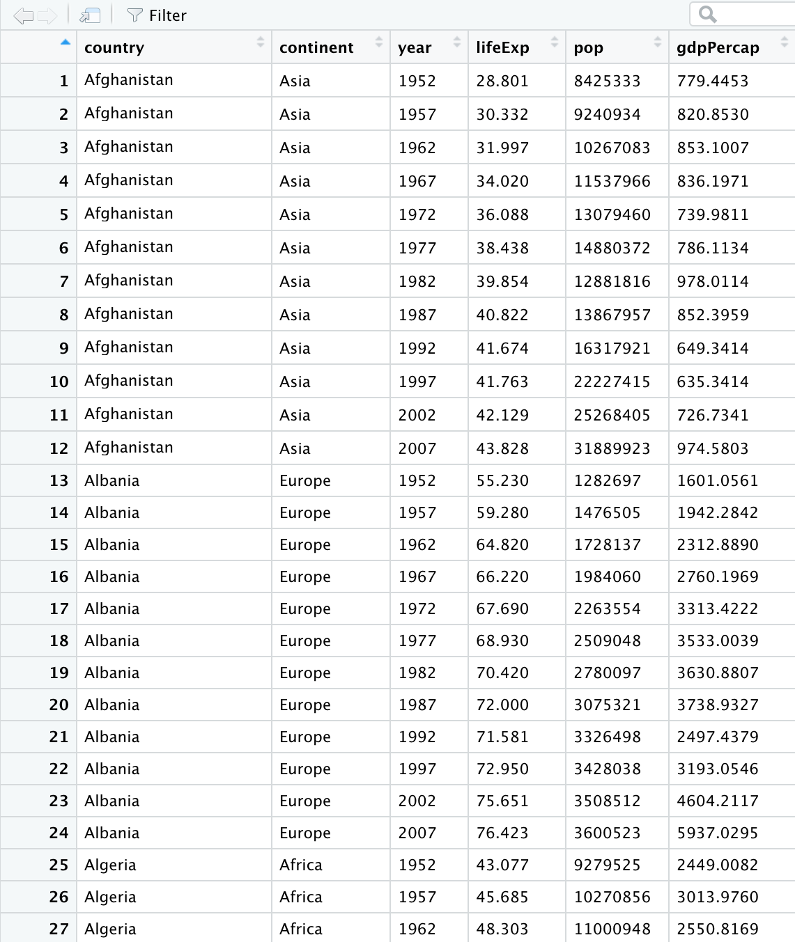 ] .pull-right[ 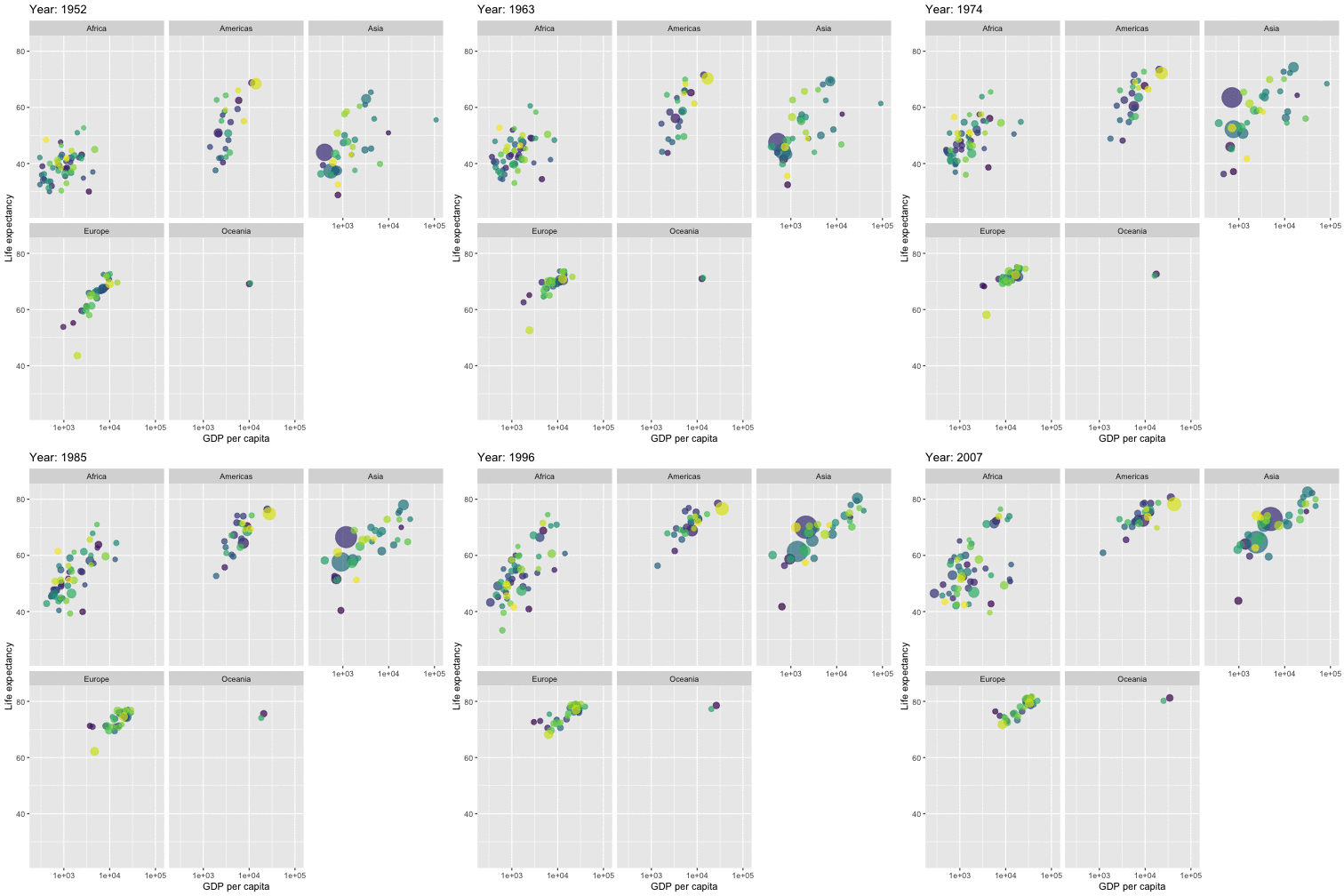<!-- --> ] --- # Data Analysis Workflow 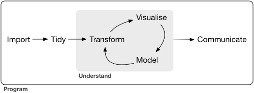 --- # Outline 1. Basics of R Programming 2. Data Import 3. Data Wrangling 4. Data Visualization --- # Outline 1. Basics of R Programming ⚙️ 2. Data Import 3. Data Wrangling 4. Data Visualization --- # What is R? - R is a software environment for statistical computing and graphics. - Language designers: **R**oss Ihaka and **R**obert Gentleman at the University of Auckland, New Zealand. - Parent language: S - The latest R version 4.0.1 has been released on 2020-06-06.  --- # Why R? - **Free** - **Powerful:** Over 14600 contributed packages on the main repository (CRAN), as of July 2019, provided by top international researchers and programmers. - **Flexible:** It is a language, and thus allows you to create your own solutions. - **Community:** Large global community friendly and helpful, lots of resources. --- background-image: url('renv.png') background-position: center background-size: contain ## R environment --- background-image: url('rstudio1.png') background-position: center background-size: contain ## The RStudio IDE --- background-image: url('rstudio2.png') background-position: center background-size: contain ## The RStudio IDE .footer-note[.tiny[.green[Image Credit: ][Clastic Detritus ](https://clasticdetritus.com/2013/01/10/creating-data-plots-with-r/)]] --- background-image: url('rstudioanalogy.jpeg') background-position: center background-size: contain ## The RStudio IDE .footer-note[.tiny[.green[Image Credit: ]R-Ladies Newcastle ]]] --- background-image: url('airport.jpg') background-position: center background-size: cover .content-box-yellow[ ## R and RStudio ] .footer-note[.tiny[.green[Image Credit: ][Clastic Detritus ](https://clasticdetritus.com/2013/01/10/creating-data-plots-with-r/)]] --- background-image: url('airport.jpg') background-position: center background-size: cover .content-box-yellow[ ## R and RStudio "If R were **an airplane**, RStudio would be **the airport**, providing many, many supporting services that make it easier for you, the pilot, to take off and go to awesome places. Sure, you can fly an airplane without an airport, but having those runways and supporting infrastructure is a game-changer." -- Julie Lowndes] .footer-note[.tiny[.green[Image Credit: ][Clastic Detritus ](https://clasticdetritus.com/2013/01/10/creating-data-plots-with-r/)]] --- class: inverse, center, middle # Create a new project --- background-image: url('project1.png') background-position: center background-size: contain --- background-image: url('project2.png') background-position: center background-size: contain --- background-image: url('project3.png') background-position: center background-size: contain --- background-image: url('project4.png') background-position: center background-size: contain --- background-image: url('project5.png') background-position: center background-size: contain --- background-image: url('project6.png') background-position: center background-size: contain --- ## R Console ```r 7+1 ``` ``` [1] 8 ``` ```r rnorm(10) ``` ``` [1] 0.42886236 0.87398624 -0.14720398 1.29780260 0.09344244 1.44028046 [7] 0.73037732 -1.11167627 0.50529457 0.69291615 ``` -- ## Variable assignment ```r a <- rnorm(10) a ``` ``` [1] -0.9555159 -0.5979601 -1.0782460 1.0624732 0.2590546 0.2246372 [7] -0.6120881 0.6849044 2.4574333 0.8701314 ``` -- ```r b <- a*100 b ``` ``` [1] -95.55159 -59.79601 -107.82460 106.24732 25.90546 22.46372 [7] -61.20881 68.49044 245.74333 87.01314 ``` --- # Data permanency - `ls()` can be used to display the names of the objects which are currently stored within R. - The collection of objects currently stored is called the **workspace**. ```r ls() ``` ``` [1] "a" "b" "p" ``` -- - To remove objects the function `rm` is available. - remove all objects `rm(list=ls())` - remove specific objects `rm(x, y, z)` ```r rm(a) ls() ``` ``` [1] "b" "p" ``` ```r rm(list=ls()) ls() ``` ``` character(0) ``` --- background-image: url('project7.png') background-position: center background-size: cover -- .pull-left[.full-width[.content-box-yellow[At the end of an R session, if **save**: the objects are written to a file called .RData in the current directory, and the command lines used in the session are saved to a file called .Rhistory]]] --- background-image: url('p81.png') background-position: center background-size: cover .pull-left[.full-width[.content-box-yellow[When R is started at later time **from the same directory** ]]] --- background-image: url('p82.png') background-position: center background-size: cover .pull-left[.full-width[.content-box-yellow[When R is started at later time **from the same directory** it reloads the **associated workspace** and **commands history.**]]] --- background-image: url('project9.png') background-position: center background-size: cover -- .pull-left[.full-width[.content-box-yellow[When R is started at later time **from the same directory** it reloads the **associated workspace** and **commands history.**]]] --- ## Comment your code - Each line of a comment should begin with the comment symbol and a single space: # . ```r rnorm(10) # This is a comment ``` ``` [1] -0.7146212 -0.6647724 -0.4563877 -0.3020826 0.9044316 0.7319009 [7] -2.1557290 -0.7404257 1.2983685 1.0892268 ``` ```r sum(1:10) # 1+2 ``` ``` [1] 55 ``` --- ## Style Guide - Good coding style is like correct punctuation: you can manage without it, butitsuremakesthingseasiertoread. -- Hadley Wickham ```r sum(1:10)#Bad commenting style ``` ``` [1] 55 ``` ```r sum(1:10) # Good commenting style ``` ``` [1] 55 ``` - Also, use commented lines of - and = to break up your file into easily readable sub-sections. ```r # Read data ---------------- # Plot data ---------------- ``` To learn more read Hadley Wickham's [Style guide](http://adv-r.had.co.nz/Style.html). --- ## Objects in R - R is an [object-oriented language](https://en.wikipedia.org/wiki/Object-oriented_programming). -- - An object in R is anything (data structures, functions, etc., that can be assigned to a variable). -- Let's take a look of some common types of objects. -- 1. .red[Data structures] are the ways of arranging data. - You can create objects, using the left pointing arrow <- -- 1. .red[Functions] tell R to do something. - A function may be applied to an object. - Result of applying a function is usually an object too. - All function calls need to be followed by parentheses. ```r a <- 1:20 # data structure sum(a) # sum is a function applied on a ``` ``` [1] 210 ``` ```r help.start() # Some functions work on their own. ``` --- # Getting help with functions and features - R has inbuilt help facility ### Method 1 ```r help(rnorm) ``` - For a feature specified by special characters such as `for`, `if`, `[[` ```r help("[[") ``` - Search the help files for a word or phrase. ```r help.search(‘weighted mean’) ``` ### Method 2 ```r ?rnorm ``` ```r ??rnorm ``` --- background-image: url('dataStructures.png') background-position: center background-size: contain ## Data structures .footer-note[.tiny[.green[Image Credit: ][venus.ifca.unican.es](http://venus.ifca.unican.es/Rintro/dataStruct.html)]] --- background-image: url('dataStructures.png') background-position: center background-size: contain ## Data structures .content-box-yellow[Data structures differ in terms of, - Type of data they can hold - How they are created - Structural complexity - Notation to identify and access individual elements ] .footer-note[.tiny[.green[Image Credit: ][venus.ifca.unican.es](http://venus.ifca.unican.es/Rintro/dataStruct.html)]] --- background-image: url('horse.png') background-position: center background-size: cover --- class: duke-green, center, middle # 1. Vectors --- # Vectors - Vectors are one-dimensional arrays that can hold numeric data, character data, or logical data. - Combine function c() is used to form the vector. - Data in a vector must only be one type or mode (numeric, character, or logical). You can’t mix modes in the same vector. ## Vector assignment **Syntax** ```r vector_name <- c(element1, element2, element3) ``` ```r x <- c(5, 6, 3, 1 , 100) ``` - assignment operator ('<-'), '=' can be used as an alternative. - `c()` function .red[What will be the output of the following code?] ```r y <- c(x, 500, 600) ``` --- # Types and tests with vectors ```r first_vec <- c(10, 20, 50, 70) second_vec <- c("Jan", "Feb", "March", "April") third_vec <- c(TRUE, FALSE, TRUE, TRUE) fourth_vec <- c(10L, 20L, 50L, 70L) ``` To check if it is a - vector: `is.vector()` ```r is.vector(first_vec) ``` ``` [1] TRUE ``` - character vector: `is.character()` ```r is.character(first_vec) ``` ``` [1] FALSE ``` --- - double: `is.double()` ```r is.double(first_vec) ``` ``` [1] TRUE ``` - integer: `is.integer()` ```r is.integer(first_vec) ``` ``` [1] FALSE ``` - logical: `is.logical()` ```r is.logical(first_vec) ``` ``` [1] FALSE ``` - length ```r length(first_vec) ``` ``` [1] 4 ``` --- # Coercion Vectors must be homogeneous. When you attempt to combine different types they will be coerced to the most flexible type so that every element in the vector is of the same type. Order from least to most flexible `logical` --> `integer` --> `double` --> `character` ```r a <- c(3.1, 2L, 3, 4, "GPA") typeof(a) ``` ``` [1] "character" ``` ```r anew <- c(3.1, 2L, 3, 4) typeof(anew) ``` ``` [1] "double" ``` --- ### Explicit coercion Vectors can be explicitly coerced from one class to another using the `as.*` functions, if available. For example, `as.character`, `as.numeric`, `as.integer`, and `as.logical`. ```r vec1 <- c(TRUE, FALSE, TRUE, TRUE) typeof(vec1) ``` ``` [1] "logical" ``` ```r vec2 <- as.integer(vec1) typeof(vec2) ``` ``` [1] "integer" ``` ```r vec2 ``` ``` [1] 1 0 1 1 ``` .red[Why does the below output NAs?] ```r x <- c("a", "b", "c") as.numeric(x) ``` ``` Warning: NAs introduced by coercion ``` ``` [1] NA NA NA ``` --- ```r x1 <- 1:3 x2 <- c(10, 20, 30) combinedx1x2 <- c(x1, x2) combinedx1x2 ``` ``` [1] 1 2 3 10 20 30 ``` -- ```r class(x1) ``` ``` [1] "integer" ``` ```r class(x2) ``` ``` [1] "numeric" ``` ```r class(combinedx1x2) ``` ``` [1] "numeric" ``` -- - If you combine a numeric vector and a character vector ```r y1 <- c(1, 2, 3) y2 <- c("a", "b", "c") c(y1, y2) ``` ``` [1] "1" "2" "3" "a" "b" "c" ``` --- ### Simplifying vector creation - colon `:` produces regular spaced ascending or descending sequences. ```r 10:16 ``` ``` [1] 10 11 12 13 14 15 16 ``` ```r -0.5:8.5 ``` ``` [1] -0.5 0.5 1.5 2.5 3.5 4.5 5.5 6.5 7.5 8.5 ``` -- - sequence: `seq(initial_value, final_value, increment)` ```r seq(1,11) ``` ``` [1] 1 2 3 4 5 6 7 8 9 10 11 ``` ```r seq(1, 11, length.out=5) ``` ``` [1] 1.0 3.5 6.0 8.5 11.0 ``` ```r seq(0, 11, by=2) ``` ``` [1] 0 2 4 6 8 10 ``` --- - repeats `rep()` ```r rep(9, 5) ``` ``` [1] 9 9 9 9 9 ``` ```r rep(1:4, 2) ``` ``` [1] 1 2 3 4 1 2 3 4 ``` ```r rep(1:4, each=2) # each element is repeated twice ``` ``` [1] 1 1 2 2 3 3 4 4 ``` ```r rep(1:4, times=2) # whole sequence is repeated twice ``` ``` [1] 1 2 3 4 1 2 3 4 ``` ```r rep(1:4, each=2, times=3) ``` ``` [1] 1 1 2 2 3 3 4 4 1 1 2 2 3 3 4 4 1 1 2 2 3 3 4 4 ``` ```r rep(1:4, 1:4) ``` ``` [1] 1 2 2 3 3 3 4 4 4 4 ``` ```r rep(1:4, c(4, 1, 4, 2)) ``` ``` [1] 1 1 1 1 2 3 3 3 3 4 4 ``` --- ## Logical operators ```r c(1, 2, 3) == c(10, 20, 3) ``` ``` [1] FALSE FALSE TRUE ``` ```r c(1, 2, 3) != c(10, 20, 3) ``` ``` [1] TRUE TRUE FALSE ``` ```r 1:5 > 3 ``` ``` [1] FALSE FALSE FALSE TRUE TRUE ``` ```r 1:5 < 3 ``` ``` [1] TRUE TRUE FALSE FALSE FALSE ``` - `<=` less than or equal to - `>=` greater than or equal to - `|` or - `&` and --- # Operators: `%in%` - in the set ```r a <- c(1, 2, 3) b <- c(1, 10, 3) a%in%b ``` ``` [1] TRUE FALSE TRUE ``` ```r x <- 1:10 y <- 1:3 x ``` ``` [1] 1 2 3 4 5 6 7 8 9 10 ``` ```r y ``` ``` [1] 1 2 3 ``` ```r x %in% y ``` ``` [1] TRUE TRUE TRUE FALSE FALSE FALSE FALSE FALSE FALSE FALSE ``` ```r y %in% x ``` ``` [1] TRUE TRUE TRUE ``` --- ## Vector arithmetic - operations are performed element by element. ```r c(10, 100, 100) + 2 # two is added to every element in the vector ``` ``` [1] 12 102 102 ``` -- - operations between two vectors ```r v1 <- c(1, 2, 3); v2 <- c(10, 100, 1000) v1 + v2 ``` ``` [1] 11 102 1003 ``` -- Add two vectors of unequal length ```r longvec <- seq(10, 100, length=10); shortvec <- c(1, 2, 3, 4, 5) shortvec + longvec ``` ``` [1] 11 22 33 44 55 61 72 83 94 105 ``` .red[What will be the output of the following code?] ```r first <- c(1, 2, 3, 4); second <- c(10, 100) first * second ``` --- # Missing values Use `NA` or `NaN` to place a missing value in a vector. ```r z <- c(10, 101, 2, 3, NA) is.na(z) ``` ``` [1] FALSE FALSE FALSE FALSE TRUE ``` --- class: duke-orange, center, middle # Your turn ``` [1] 1 2 3 4 5 5 4 3 2 1 ``` R code? <div class="countdown" id="timer_5f472362" style="right:0;bottom:0;" data-warnwhen="0"> <code class="countdown-time"><span class="countdown-digits minutes">01</span><span class="countdown-digits colon">:</span><span class="countdown-digits seconds">00</span></code> </div> --- ## Vectors: Subsetting ```r myvec <- 1:20; myvec ``` ``` [1] 1 2 3 4 5 6 7 8 9 10 11 12 13 14 15 16 17 18 19 20 ``` -- ```r myvec[1] ``` ``` [1] 1 ``` -- ```r myvec[5:10] ``` ``` [1] 5 6 7 8 9 10 ``` -- ```r myvec[-1] ``` ``` [1] 2 3 4 5 6 7 8 9 10 11 12 13 14 15 16 17 18 19 20 ``` -- ```r myvec[myvec > 3] ``` ``` [1] 4 5 6 7 8 9 10 11 12 13 14 15 16 17 18 19 20 ``` --- ## Vectors: Subsetting Extract elements present in vector `a` ```r a ``` ``` [1] 1 2 3 ``` ```r myvec ``` ``` [1] 1 2 3 4 5 6 7 8 9 10 11 12 13 14 15 16 17 18 19 20 ``` ```r myvec %in% a ``` ``` [1] TRUE TRUE TRUE FALSE FALSE FALSE FALSE FALSE FALSE FALSE FALSE FALSE [13] FALSE FALSE FALSE FALSE FALSE FALSE FALSE FALSE ``` ```r myvec[myvec %in% a] ``` ``` [1] 1 2 3 ``` -- ```r b <- 100:105 myvec[myvec %in% b] ``` ``` integer(0) ``` --- class: duke-orange # Your turn 1. Generate a sequence using the code `seq(from=1, to=10, by=1)`. 2. What other ways can you generate the same sequence? 3. Using the function `rep` , create the below sequence 1, 2, 3, 4, 1, 2, 3, 4, 1, 2, 3, 4 4. Extract the 5th element. 5. Extract elements greater than 2. <div class="countdown" id="timer_5f4722ba" style="right:0;bottom:0;" data-warnwhen="0"> <code class="countdown-time"><span class="countdown-digits minutes">02</span><span class="countdown-digits colon">:</span><span class="countdown-digits seconds">30</span></code> </div> --- class: duke-green, center, middle # 2. Data Frames --- background-image: url('dataStructures.png') background-position: center background-size: contain --- # Data frames - Rectangular arrangement of data with rows corresponding to observational units and columns corresponding to variables. - More general than a matrix in that different columns can contain different modes of data. - It’s similar to the datasets you’d typically see in SPSS and MINITAB. - Data frames are the most common data structure you’ll deal with in R.  .footer-note[.tiny[.green[Image Credit: ][Hadley Wickham and Garrett Grolemund](https://r4ds.had.co.nz/tidy-data.html)]] --- # Create a data frame **Syntax** ```r name_of_the_dataframe <- data.frame( var1_name=vector of values of the first variable, var2_names=vector of values of the second variable) ``` **Example** ```r corona <- data.frame(ID=c("C001", "C002", "C003", "C004"), Location=c("Beijing", "Wuhan", "Shanghai", "Beijing"), Test_Results=c(FALSE, TRUE, FALSE, FALSE)) corona ``` ``` ID Location Test_Results 1 C001 Beijing FALSE 2 C002 Wuhan TRUE 3 C003 Shanghai FALSE 4 C004 Beijing FALSE ``` To check if it is a dataframe ```r is.data.frame(corona) ``` ``` [1] TRUE ``` --- # Some useful functions with dataframes ```r colnames(corona) ``` ``` [1] "ID" "Location" "Test_Results" ``` ```r length(corona) ``` ``` [1] 3 ``` ```r dim(corona) ``` ``` [1] 4 3 ``` ```r nrow(corona) ``` ``` [1] 4 ``` ```r ncol(corona) ``` ``` [1] 3 ``` --- # Some useful functions with dataframes (cont.) ```r summary(corona) ``` ``` ID Location Test_Results Length:4 Length:4 Mode :logical Class :character Class :character FALSE:3 Mode :character Mode :character TRUE :1 ``` ```r str(corona) ``` ``` 'data.frame': 4 obs. of 3 variables: $ ID : chr "C001" "C002" "C003" "C004" $ Location : chr "Beijing" "Wuhan" "Shanghai" "Beijing" $ Test_Results: logi FALSE TRUE FALSE FALSE ``` --- # Subsetting dataframes ```r corona$Location ``` ``` [1] "Beijing" "Wuhan" "Shanghai" "Beijing" ``` ```r corona[,2] ``` ``` [1] "Beijing" "Wuhan" "Shanghai" "Beijing" ``` ```r corona[, "Location"] ``` ``` [1] "Beijing" "Wuhan" "Shanghai" "Beijing" ``` ```r corona[2, ] ``` ``` ID Location Test_Results 2 C002 Wuhan TRUE ``` --- class: duke-orange, center, middle # Your turn 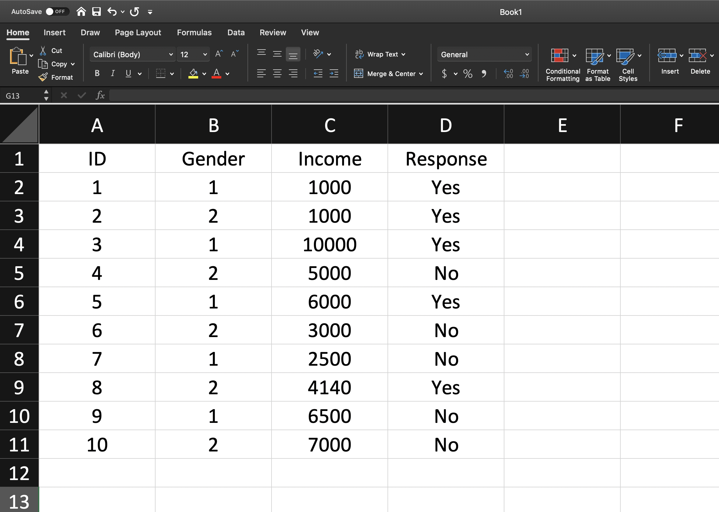 <div class="countdown" id="timer_5f472406" style="right:0;bottom:0;" data-warnwhen="0"> <code class="countdown-time"><span class="countdown-digits minutes">03</span><span class="countdown-digits colon">:</span><span class="countdown-digits seconds">30</span></code> </div> --- # Installing R Packages ## Method 1 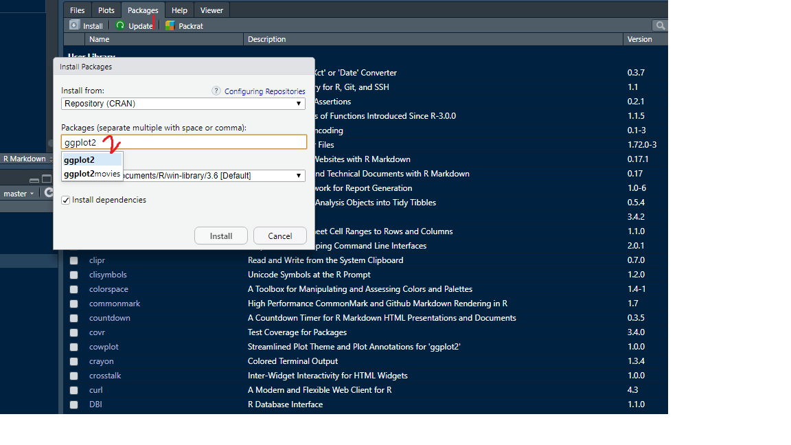 ## Method 2 ```r install.packages("ggplot2") ``` --- # install.packages vs library  .footer-note[.tiny[.green[Image Credit: Professor Di Cook Monash University, AUS ]]] --- # Built-in dataframes ```r library(gapminder) data(gapminder) head(gapminder) ``` ``` # A tibble: 6 x 6 country continent year lifeExp pop gdpPercap <fct> <fct> <int> <dbl> <int> <dbl> 1 Afghanistan Asia 1952 28.8 8425333 779. 2 Afghanistan Asia 1957 30.3 9240934 821. 3 Afghanistan Asia 1962 32.0 10267083 853. 4 Afghanistan Asia 1967 34.0 11537966 836. 5 Afghanistan Asia 1972 36.1 13079460 740. 6 Afghanistan Asia 1977 38.4 14880372 786. ``` ```r str(gapminder) ``` ``` tibble [1,704 × 6] (S3: tbl_df/tbl/data.frame) $ country : Factor w/ 142 levels "Afghanistan",..: 1 1 1 1 1 1 1 1 1 1 ... $ continent: Factor w/ 5 levels "Africa","Americas",..: 3 3 3 3 3 3 3 3 3 3 ... $ year : int [1:1704] 1952 1957 1962 1967 1972 1977 1982 1987 1992 1997 ... $ lifeExp : num [1:1704] 28.8 30.3 32 34 36.1 ... $ pop : int [1:1704] 8425333 9240934 10267083 11537966 13079460 14880372 12881816 13867957 16317921 22227415 ... $ gdpPercap: num [1:1704] 779 821 853 836 740 ... ``` --- class: duke-orange # Your turn Use the R dataset “gapminder” to answer the following questions: 1. How many rows and columns does gapminder have? 2. Extract column names in gapminder. 3. Display the first 10 rows of the data. 4. Display the last 3 rows of the data. 4. Select rows from 10 to 20, containing all variables. 5. Select rows from 10 to 20 containing `country` and `lifeExp`. 6. Create a single vector (a new object) called ‘LifeExpectancy’ containing the values in `lifeExp` in gapminder. 7. How many countries in Asia had `lifeExp` larger than 30 in 1952? <div class="countdown" id="timer_5f4723c7" style="right:0;bottom:0;" data-warnwhen="0"> <code class="countdown-time"><span class="countdown-digits minutes">05</span><span class="countdown-digits colon">:</span><span class="countdown-digits seconds">30</span></code> </div> --- # What have we learned today? --- class: center, middle All rights reserved by [Dr. Thiyanga S. Talagala](https://thiyanga.netlify.app/)