class: center, middle, inverse, title-slide # STA 506 2.0 Linear Regression Analysis ## Lecture 11-i: Transformations to Correct Model Inadequacies ### Dr Thiyanga S. Talagala ### 2020-11-07 --- ## Introduction In this section we are going to learn methods and procedures for building regression models when the assumptions are violated. ### Transformations - Variance-stabilizing transformations - Transformations to linearize the model ### How to get around the problem? - Transform `\(X\)` variable(s) - Transform `\(Y\)` - Transformations on both `\(X\)` variable(s) and `\(Y\)`. --- class: duke-orange, middle ## Variance-Stabilizing Transformations --- ## Dataset 1 We will try to model salary as a function of years of experience. ```r library(tidyverse) salarydata <- read_csv("salarydata.csv") salarydata ``` ``` # A tibble: 100 x 2 years salary <dbl> <dbl> 1 1 41504 2 1 32619 3 1 44322 4 2 40038 5 2 46147 6 2 38447 7 2 38163 8 3 42104 9 3 25597 10 3 39599 # … with 90 more rows ``` Data are obtained from: https://daviddalpiaz.github.io/appliedstats/transformations.html --- ## Salary vs Years of Experience ```r ggplot(salarydata, aes(x=years, y=salary)) + geom_point() ``` 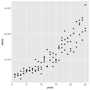<!-- --> ```r cor(salarydata$years, salarydata$salary) ``` ``` [1] 0.9133066 ``` --- ## Fit a Simple Linear Regression Model ```r salary_fit <- lm(salary ~ years, data = salarydata) summary(salary_fit) ``` ``` Call: lm(formula = salary ~ years, data = salarydata) Residuals: Min 1Q Median 3Q Max -57225 -18104 241 15589 91332 Coefficients: Estimate Std. Error t value Pr(>|t|) (Intercept) 5302 5750 0.922 0.359 years 8637 389 22.200 <2e-16 *** --- Signif. codes: 0 '***' 0.001 '**' 0.01 '*' 0.05 '.' 0.1 ' ' 1 Residual standard error: 27360 on 98 degrees of freedom Multiple R-squared: 0.8341, Adjusted R-squared: 0.8324 F-statistic: 492.8 on 1 and 98 DF, p-value: < 2.2e-16 ``` --- ## Compute Residuals and Fitted Values ```r library(broom) salary_residuals <- augment(salary_fit) salary_residuals ``` ``` # A tibble: 100 x 8 salary years .fitted .resid .std.resid .hat .sigma .cooksd <dbl> <dbl> <dbl> <dbl> <dbl> <dbl> <dbl> <dbl> 1 41504 1 13939. 27565. 1.03 0.0391 27347. 0.0215 2 32619 1 13939. 18680. 0.697 0.0391 27428. 0.00988 3 44322 1 13939. 30383. 1.13 0.0391 27315. 0.0261 4 40038 2 22575. 17463. 0.650 0.0345 27436. 0.00753 5 46147 2 22575. 23572. 0.877 0.0345 27388. 0.0137 6 38447 2 22575. 15872. 0.590 0.0345 27447. 0.00622 7 38163 2 22575. 15588. 0.580 0.0345 27449. 0.00600 8 42104 3 31212. 10892. 0.404 0.0302 27473. 0.00255 9 25597 3 31212. -5615. -0.208 0.0302 27490. 0.000677 10 39599 3 31212. 8387. 0.311 0.0302 27482. 0.00151 # … with 90 more rows ``` --- ## Residuals vs Fitted Values ```r ggplot(salary_residuals, aes(x=.fitted, y=.resid)) + geom_point() ``` 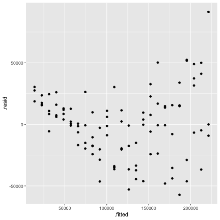<!-- --> --- ## Normality assumption .pull-left[ ```r qplot(data=salary_residuals, x=.resid,)+ geom_histogram(color="black", fill="lightblue") ``` 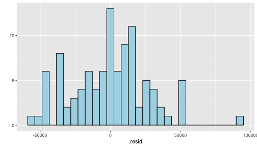<!-- --> ```r shapiro.test(salary_residuals$.resid) ``` ``` Shapiro-Wilk normality test data: salary_residuals$.resid W = 0.98258, p-value = 0.2101 ``` ] .pull-right[ ```r ggplot(salary_residuals, aes(sample=.resid))+ stat_qq() + stat_qq_line() + labs(x="Theoretical Quantiles", y="Sample Quantiles") ``` 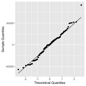<!-- --> ] --- ## Variance - Stabilizing Transformations .pull-left[ <!-- --> ] .pull-left[ - Useful variance-stabilizing transformations - square root: `\(\sqrt{y}\)` - log transformation: `\(log(y)\)` - reciprocal: `\(y^{-1}\)` - reciprocal square root: `\(y^{-1/2}\)` ] --- ## Apply log transformation `$$log(Y) = \beta_0 + \beta_1x_ + \epsilon$$` ```r salarydata$log.salary <- log(salarydata$salary) salarydata ``` ``` # A tibble: 100 x 3 years salary log.salary <dbl> <dbl> <dbl> 1 1 41504 10.6 2 1 32619 10.4 3 1 44322 10.7 4 2 40038 10.6 5 2 46147 10.7 6 2 38447 10.6 7 2 38163 10.5 8 3 42104 10.6 9 3 25597 10.2 10 3 39599 10.6 # … with 90 more rows ``` --- ## Fit a regression model with log transformation ```r salary_fit_log <- lm(log.salary ~ years, data = salarydata) salary_fit_log ``` ``` Call: lm(formula = log.salary ~ years, data = salarydata) Coefficients: (Intercept) years 10.48381 0.07888 ``` --- ## Compute Residuals and Fitted values ```r salary_log_residuals <- augment(salary_fit_log) salary_log_residuals ``` ``` # A tibble: 100 x 8 log.salary years .fitted .resid .std.resid .hat .sigma .cooksd <dbl> <dbl> <dbl> <dbl> <dbl> <dbl> <dbl> <dbl> 1 10.6 1 10.6 0.0709 0.370 0.0391 0.196 0.00278 2 10.4 1 10.6 -0.170 -0.887 0.0391 0.196 0.0160 3 10.7 1 10.6 0.137 0.713 0.0391 0.196 0.0103 4 10.6 2 10.6 -0.0440 -0.229 0.0345 0.196 0.000936 5 10.7 2 10.6 0.0980 0.510 0.0345 0.196 0.00465 6 10.6 2 10.6 -0.0845 -0.440 0.0345 0.196 0.00346 7 10.5 2 10.6 -0.0919 -0.479 0.0345 0.196 0.00409 8 10.6 3 10.7 -0.0725 -0.377 0.0302 0.196 0.00221 9 10.2 3 10.7 -0.570 -2.96 0.0302 0.187 0.137 10 10.6 3 10.7 -0.134 -0.696 0.0302 0.196 0.00754 # … with 90 more rows ``` --- ## Residuals vs Fitted values <!-- --> --- ## Residuals vs Fitted .pull-left[ `$$Y = \beta_0 + \beta_1x + \epsilon$$` <!-- --> ] .pull-right[ `$$log(Y) = \beta_0 + \beta_1x + \epsilon$$` <!-- --> ] --- ## Normality assumption `\(log(Y) = \beta_0 + \beta_1x + \epsilon\)` ```r qplot(data=salary_log_residuals, x=.resid,)+ geom_histogram(color="black", fill="lightblue") ``` <!-- --> --- ## Normality assumption (cont.) ```r ggplot(salary_log_residuals, aes(sample=.resid))+ stat_qq() + stat_qq_line() + labs(x="Theoretical Quantiles", y="Sample Quantiles") ``` <!-- --> --- ## Normality assumption (cont.) ```r shapiro.test(salary_log_residuals$.resid) ``` ``` Shapiro-Wilk normality test data: salary_log_residuals$.resid W = 0.98033, p-value = 0.141 ``` --- ## Model Statistics ```r summary(salary_fit_log) ``` ``` Call: lm(formula = log.salary ~ years, data = salarydata) Residuals: Min 1Q Median 3Q Max -0.57022 -0.13560 0.03048 0.14157 0.41366 Coefficients: Estimate Std. Error t value Pr(>|t|) (Intercept) 10.48381 0.04108 255.18 <2e-16 *** years 0.07888 0.00278 28.38 <2e-16 *** --- Signif. codes: 0 '***' 0.001 '**' 0.01 '*' 0.05 '.' 0.1 ' ' 1 Residual standard error: 0.1955 on 98 degrees of freedom Multiple R-squared: 0.8915, Adjusted R-squared: 0.8904 F-statistic: 805.2 on 1 and 98 DF, p-value: < 2.2e-16 ``` --- ## Hypothesis testing ### Intercept `\(H_0: \beta_0 = 0\)` vs `\(H_1: \beta_0 \neq 0\)` Decision: p-value < 0.05. We reject `\(H_0\)` under 0.05 level of significance. Conclusion: We can conclude that population regression line intercept is significantly different from 0. ### Slope `\(H_0: \beta_1 = 0\)` vs `\(H_1: \beta_1 \neq 0\)` Decision: p-value < 0.05. We reject `\(H_0\)` under 0.05 level of significance. Conclusion: The variable `years` contributes significantly to the model. --- # Re-scale ### log scale to the original scale of the data **Preliminary Maths** `$$Y=10$$` `$$log(10) = 2.302585$$` `$$e^{2.302585} = 10$$` `$$e^{a+b} = e^ae^b$$` ### New fitted regression model `$$\hat{log(Y)} = 10.48 + 0.079X$$` Convert to original scale `$$e^{\hat{log(Y)}} = e^{10.48 + 0.079X}$$` `$$\hat{Y} = e^{10.48}e^{0.079X}$$` --- ## Interpretation of slope When `\(X=x_1\)` `$$Y' = e^{10.48}e^{0.079x_1}$$` When `\(X={x_1 + 1}\)` `$$Y'' = e^{10.48}e^{0.079(x_1 + 1)} = e^{10.48}e^{0.079(x_1)}e^{0.079}$$` `$$e^{0.079} = 1.0822$$` We see that for every one additional year of experience, average (median) salary increases 1.0822 times. We are now multiplying, not adding. --- ## Interpretation of slope `$$\hat{log(Y)} = \hat{\beta_0} + \hat{\beta_1}x$$` ### Interpretation of `\(\hat{\beta_0}\)` When `\(x=0\)`, the median of `\(Y\)` is expected to be `\(e^{\hat{\beta}_0}\)`. ### Interpretation of `\(\hat{\beta_1}\)` For every one unit increase in `\(x\)`, the median of `\(Y\)` is expected to multiply by a factor of `\(e^{\hat{\beta}_1}\)`. Why median not mean?: Read here https://www2.stat.duke.edu/courses/Spring20/sta210.001/slides/lec-slides/09-transformations.html#29 --- ## Confidence interval for `\(\beta_j\)` The confidence interval for the coefficient of `\(x\)` describing its relationship with `\(Y\)` is: - Confidence intervals `\(\beta_0\)` `$$[\hat{\beta_0} - t_{\alpha/2, n-2}se(\hat{\beta_0}), \hat{\beta_0} + t_{\alpha/2, n-2}se(\hat{\beta_0})]$$` - Confidence intervals `\(\beta_1\)` `$$[\hat{\beta_1} - t_{\alpha/2, n-2}se(\hat{\beta_1}), \hat{\beta_1} + t_{\alpha/2, n-2}se(\hat{\beta_1})]$$` ```r confint(salary_fit_log, level=0.95) ``` ``` 2.5 % 97.5 % (Intercept) 10.40227614 10.56533628 years 0.07336341 0.08439611 ``` --- ## Confidence interval for `\(\beta_j\)` - backtransform The confidence interval for the coefficient of `\(x\)` describing its relationship with `\(log(Y)\)` is: - Confidence intervals `\(\beta_0\)` `$$[e^{\hat{\beta_0} - t_{\alpha/2, n-2}se(\hat{\beta_0})}, e^{\hat{\beta_0} + t_{\alpha/2, n-2}se(\hat{\beta_0})}]$$` - Confidence intervals `\(\beta_1\)` `$$[e^{\hat{\beta_1} - t_{\alpha/2, n-2}se(\hat{\beta_1})}, e^{\hat{\beta_1} + t_{\alpha/2, n-2}se(\hat{\beta_1})}]$$` ```r exp(confint(salary_fit_log, level=0.95)) ``` ``` 2.5 % 97.5 % (Intercept) 32934.503906 38767.45083 years 1.076122 1.08806 ``` --- class: duke-orange, middle ## Transformations to Linearize the Model <!--https://ademos.people.uic.edu/Chapter12.html--> ---  source: https://srilankamirror.com/biz/20026-coconuts-to-be-measured-by-weight-instead-of-circumference --- ## Data ```r coconut <- read_csv("coconut.csv") # Ignore the warning message coconut ``` ``` # A tibble: 100 x 3 X1 weight circumference <dbl> <dbl> <dbl> 1 1 773. 27.8 2 2 772. 27.8 3 3 780. 27.9 4 4 790. 28.1 5 5 806. 28.4 6 6 813. 28.5 7 7 817. 28.6 8 8 820. 28.6 9 9 818. 28.6 10 10 830. 28.8 # … with 90 more rows ``` --- ## EDA .pull-left[ ```r qplot(data=coconut, y=weight, geom=c("boxplot"))+ geom_boxplot(color="black", fill="#d95f02") ``` 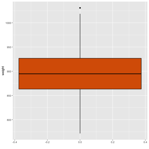<!-- --> ] .pull-right[ ```r qplot(data=coconut, y=circumference, geom=c("boxplot"))+ geom_boxplot(color="black", fill="forestgreen") ``` 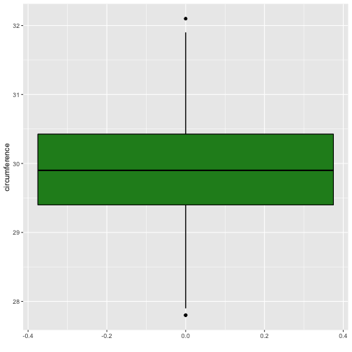<!-- --> ] --- ## Weight vs Circumference ```r ggplot(coconut, aes(x=circumference, y=weight)) + geom_point() ``` 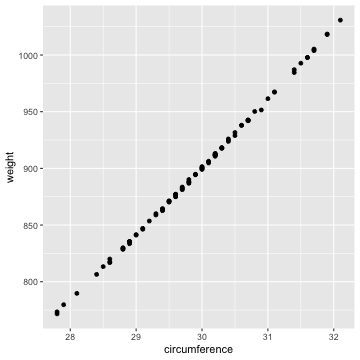<!-- --> ```r cor(coconut$circumference, coconut$weight) ``` ``` [1] 0.9996482 ``` --- # Fit a regression model ```r coconut.lm <- lm(weight ~ circumference, data=coconut) coconut.lm ``` ``` Call: lm(formula = weight ~ circumference, data = coconut) Coefficients: (Intercept) circumference -897.25 59.94 ``` --- ## Compute Residuals and Fitted Values ```r coconut.lm.result <- broom::augment(coconut.lm) coconut.lm.result ``` ``` # A tibble: 100 x 8 weight circumference .fitted .resid .std.resid .hat .sigma .cooksd <dbl> <dbl> <dbl> <dbl> <dbl> <dbl> <dbl> <dbl> 1 773. 27.8 769. 4.32 2.93 0.0602 1.46 0.275 2 772. 27.8 769. 2.57 1.74 0.0602 1.50 0.0971 3 780. 27.9 775. 4.62 3.12 0.0556 1.45 0.287 4 790. 28.1 787. 2.63 1.77 0.0470 1.50 0.0772 5 806. 28.4 805. 1.39 0.934 0.0359 1.52 0.0162 6 813. 28.5 811. 2.25 1.50 0.0326 1.51 0.0380 7 817. 28.6 817. -0.247 -0.165 0.0295 1.53 0.000413 8 820. 28.6 817. 2.98 1.99 0.0295 1.50 0.0601 9 818. 28.6 817. 0.473 0.316 0.0295 1.53 0.00152 10 830. 28.8 829. 0.825 0.549 0.0240 1.53 0.00371 # … with 90 more rows ``` --- ## Residuals vs Fitted values 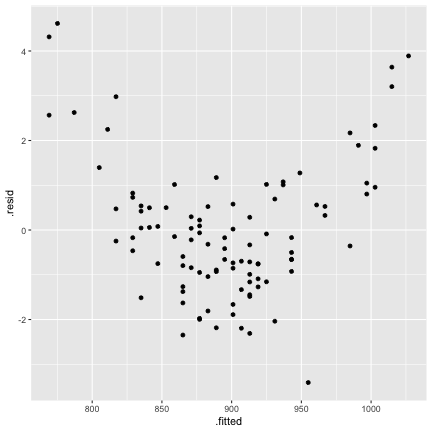<!-- --> --- ## Normality assumption ```r qplot(data=coconut.lm.result, x=.resid, geom=c("histogram"))+ geom_histogram(color="black", fill="#d95f02") ``` 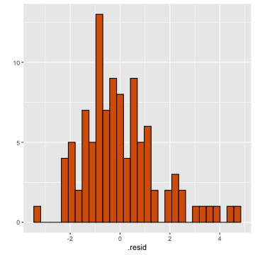<!-- --> --- ## Normality assumption ```r ggplot(coconut.lm.result, aes(sample=.resid))+ stat_qq() + stat_qq_line() + labs(x="Theoretical Quantiles", y="Sample Quantiles") ``` <!-- --> --- ## Normality assumption (cont.) ```r shapiro.test(coconut.lm.result$.resid) ``` ``` Shapiro-Wilk normality test data: coconut.lm.result$.resid W = 0.95463, p-value = 0.001697 ``` --- ## Transform Y `$$\sqrt(Y) = \beta_0 + \beta_1 x + \epsilon$$` ```r coconut$sqrt.weight <- sqrt(coconut$weight) coconut ``` ``` # A tibble: 100 x 4 X1 weight circumference sqrt.weight <dbl> <dbl> <dbl> <dbl> 1 1 773. 27.8 27.8 2 2 772. 27.8 27.8 3 3 780. 27.9 27.9 4 4 790. 28.1 28.1 5 5 806. 28.4 28.4 6 6 813. 28.5 28.5 7 7 817. 28.6 28.6 8 8 820. 28.6 28.6 9 9 818. 28.6 28.6 10 10 830. 28.8 28.8 # … with 90 more rows ``` --- ### Estimate parameters of `\(\sqrt(Y) = \beta_0 + \beta_1 x + \epsilon\)` ```r coconut.lm2 <- lm(sqrt.weight ~ circumference, data=coconut) coconut.lm2 ``` ``` Call: lm(formula = sqrt.weight ~ circumference, data = coconut) Coefficients: (Intercept) circumference 0.01631 0.99951 ``` --- ## Compute Residuals and Fitted Values ```r coconut.lm.result2 <- broom::augment(coconut.lm2) coconut.lm.result2 ``` ``` # A tibble: 100 x 8 sqrt.weight circumference .fitted .resid .std.resid .hat .sigma .cooksd <dbl> <dbl> <dbl> <dbl> <dbl> <dbl> <dbl> <dbl> 1 27.8 27.8 27.8 0.00810 0.536 0.0602 0.0157 9.20e-3 2 27.8 27.8 27.8 -0.0234 -1.55 0.0602 0.0155 7.66e-2 3 27.9 27.9 27.9 0.0211 1.39 0.0556 0.0155 5.69e-2 4 28.1 28.1 28.1 -0.000372 -0.0244 0.0470 0.0157 1.47e-5 5 28.4 28.4 28.4 -0.00373 -0.244 0.0359 0.0157 1.10e-3 6 28.5 28.5 28.5 0.0166 1.08 0.0326 0.0156 1.98e-2 7 28.6 28.6 28.6 -0.0221 -1.43 0.0295 0.0155 3.13e-2 8 28.6 28.6 28.6 0.0343 2.23 0.0295 0.0153 7.58e-2 9 28.6 28.6 28.6 -0.00946 -0.615 0.0295 0.0157 5.75e-3 10 28.8 28.8 28.8 0.00562 0.365 0.0240 0.0157 1.64e-3 # … with 90 more rows ``` --- ## Residuals vs Fitted values ```r ggplot(coconut.lm.result2, aes(x=.fitted, y=.resid)) + geom_point() ``` <!-- --> --- ## Residuals vs Fitted values .pull-left[ `\(Y = \beta_0 + \beta_1 x + \epsilon\)` <!-- --> ] .pull-right[ `\(\sqrt(Y) = \beta_0 + \beta_1 x + \epsilon\)` 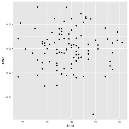<!-- --> ] --- ## Normality assumption ```r qplot(data=coconut.lm.result2, x=.resid, geom=c("histogram"))+ geom_histogram(color="black", fill="#d95f02") ``` 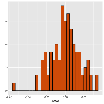<!-- --> --- ## Normality assumption ```r ggplot(coconut.lm.result2, aes(sample=.resid))+ stat_qq() + stat_qq_line() + labs(x="Theoretical Quantiles", y="Sample Quantiles") ``` <!-- --> --- ## Normality assumption (cont.) ```r shapiro.test(coconut.lm.result2$.resid) ``` ``` Shapiro-Wilk normality test data: coconut.lm.result2$.resid W = 0.98624, p-value = 0.3885 ``` --- ## Normality test .pull-left[ `\(Y = \beta_0 + \beta_1 x + \epsilon\)` 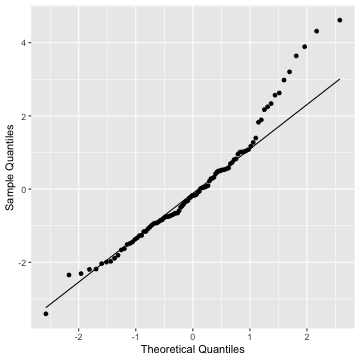<!-- --> ``` Shapiro-Wilk normality test data: coconut.lm.result$.resid W = 0.95463, p-value = 0.001697 ``` ] .pull-right[ `\(\sqrt(Y) = \beta_0 + \beta_1 x + \epsilon\)` <!-- --> ``` Shapiro-Wilk normality test data: coconut.lm.result2$.resid W = 0.98624, p-value = 0.3885 ``` ] --- ### Your turn: Tests on individual regression coefficients ```r summary(coconut.lm2) ``` ``` Call: lm(formula = sqrt.weight ~ circumference, data = coconut) Residuals: Min 1Q Median 3Q Max -0.054212 -0.009988 0.000234 0.008474 0.034324 Coefficients: Estimate Std. Error t value Pr(>|t|) (Intercept) 0.016311 0.049346 0.331 0.742 circumference 0.999507 0.001648 606.382 <2e-16 *** --- Signif. codes: 0 '***' 0.001 '**' 0.01 '*' 0.05 '.' 0.1 ' ' 1 Residual standard error: 0.0156 on 98 degrees of freedom Multiple R-squared: 0.9997, Adjusted R-squared: 0.9997 F-statistic: 3.677e+05 on 1 and 98 DF, p-value: < 2.2e-16 ``` --- ## Back transformation: sqrt - The back transformation is to square the number. If you have negative numbers, you can't take the square root; you should add a constant to each number to make them all positive. - Square-root transformation when the variable is a count of something, or the variables that can take positive values. --- ## Back transformation: sqrt `$$\sqrt(Y) = 0.016 + 0.99x$$` `$$Y = (0.016 + 0.99x)^2$$` `$$Y = 0.016^2 + 2(0.016 \times0.99)x + (0.99x)^2$$` > "Although the popular square root transformation can be useful for simplifying relationships with quadratic effects, and also for stabilizing variances (Baguley, 2012), this transformation does not aid in interpretation." > Data Transformations for Inference with Linear Regression: Clarifications and Recommendations. [J. Pek, O. Wong, A. C. Wong] Link to the paper: https://scholarworks.umass.edu/cgi/viewcontent.cgi?article=1360&context=pare --- # Note - When the model is presented to the professional community or to the general public/ when making preidctions, transformations done to the dependent variable `\(Y\)` should be transformed back to the **original units** --- ## Model with transformation on X `$$\hat{Y} = \hat{\beta}_0 + \hat{\beta}_1log(x)$$` ## Interpretation of intercept: When `\(log(x)=0\)`, that is `\(x=1\)`, mean of `\(Y\)` is expected to be `\(\hat{\beta_0}\)` ## Interpretation of slope: When `\(X\)` is multiplied by a factor of `\(K\)`, the mean of `\(Y\)` changes by `\(\hat{\beta}_1log(K)\)`. Example: when `\(K=2\)` (some constant value) When `\(X\)` is multiplied by a factor of 2, the mean of `\(Y\)` changes by `\(\hat{\beta}_1log(2)\)`. --- ## Help but Not RULES ### Transformations on X - Suppose the assumption of normally and independently distributed responses with constant variance are at least approximately satisfied, however the relationship between `\(Y\)` and one or more of the regressor variables is nonlinear. ### Transformations on Y - To correct nonnormality assumption and/or nonconstant variance assumption of the error term. --- class: center, middle Acknowledgement Introduction to Linear Regression Analysis, Douglas C. Montgomery, Elizabeth A. Peck, G. Geoffrey Vining All rights reserved by [Dr. Thiyanga S. Talagala](https://thiyanga.netlify.app/)