background-image: url('orange.jpg') background-position: center background-size: cover ### What does a statistician do? --- ### What does a statistician do? ``` # A tibble: 15 × 6 country continent year lifeExp pop gdpPercap <fct> <fct> <int> <dbl> <int> <dbl> 1 Afghanistan Asia 1952 28.8 8425333 779. 2 Afghanistan Asia 1957 30.3 9240934 821. 3 Afghanistan Asia 1962 32.0 10267083 853. 4 Afghanistan Asia 1967 34.0 11537966 836. 5 Afghanistan Asia 1972 36.1 13079460 740. 6 Afghanistan Asia 1977 38.4 14880372 786. 7 Afghanistan Asia 1982 39.9 12881816 978. 8 Afghanistan Asia 1987 40.8 13867957 852. 9 Afghanistan Asia 1992 41.7 16317921 649. 10 Afghanistan Asia 1997 41.8 22227415 635. 11 Afghanistan Asia 2002 42.1 25268405 727. 12 Afghanistan Asia 2007 43.8 31889923 975. 13 Albania Europe 1952 55.2 1282697 1601. 14 Albania Europe 1957 59.3 1476505 1942. 15 Albania Europe 1962 64.8 1728137 2313. ``` --- 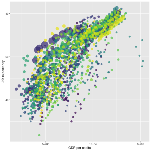<!-- --> --- <!-- --> --- ### What is Regression Analysis? - Statistical technique for investigating and modelling the relationship between variables. ### Statistical Modelling - a simplified, mathematically-formalized way to approximate reality (i.e. what generates your data) and optionally to make predictions from this approximation. --- background-image: url('regression.PNG') background-position: center background-size: contain ### Statistical Modelling: The Bigger Picture --- background-image: url('workflowds.png') background-position: center background-size: contain ### Statistical Modelling Workflow <!--https://github.com/MaximeWack/tidyflow--> .footer-note[.tiny[.green[Image Credit: ][Hadley Wickham ](https://r4ds.had.co.nz/)]] --- background-image: url('hellor.png') background-position: center background-size: contain ### Software: R and RStudio (IDE) [Visit: https://hellor.netlify.app/] --- ### Consider trying to answer the following kinds of questions: - To use the parents’ heights to predict childrens’ heights. .pull-left[ ``` mheight dheight 1 59.7 55.1 2 58.2 56.5 3 60.6 56.0 4 60.7 56.8 5 61.8 56.0 6 55.5 57.9 ``` ] .pull-right[ <!-- --> ] Predict the daughter's height if her mother's height is 66 inches? --- background-image: url('calculator.png') background-position: right background-size: contain --- background-image: url('curvefitting.jpg') background-position: right background-size: contain .pull-left[ - Regression Analysis involves curve fitting. - **Curve fitting:** The process of finding a relation or equation of **best fit**. ] --- # Model <!--https://www2.stat.duke.edu/courses/Spring19/sta210.001/slides/lec-slides/01-regression-intro.html#18--> `$$Y = f(x_1, x_2, x_3) + \epsilon$$` > Goal: Estimate `\(f\)` ? ## How do we estimate `\(f\)`? ### Non-parametric methods: estimate `\(f\)` using observed data without making explicit assumptions about the functional form of `\(f\)`. ### Parametric methods estimate `\(f\)` using observed data by making assumptions about the functional form of `\(f\)`. Ex: `\(Y = \beta_0 + \beta_1x_1 + \beta_2x_2 + \beta_3x_3 + \epsilon\)` --- background-image: url('regressionpaper1.png') background-position: center background-size: contain --- background-image: url('regressionpaper2.png') background-position: center background-size: contain --- background-image: url('regressionpaper3.png') background-position: center background-size: contain --- ## Do not under-estimate the power of simple models. <iframe width="560" height="315" src="https://www.youtube.com/embed/1zX6diCwlZA" frameborder="0" allow="accelerometer; autoplay; encrypted-media; gyroscope; picture-in-picture" allowfullscreen></iframe> <!--https://www.linkedin.com/feed/update/urn:li:activity:6489030516644380672/--> -- - Create something new which is more efficient than the existing method. --- background-image: url('GDPR.jpg') background-position: center background-size: contain --- ## Machine Learning Algorithms .pull-left[ 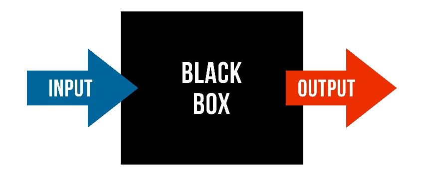 ] .pull-right[  ] -- - Random Forest - XGboost - Neural networks, etc. --- ## Pearson's Correlation Coefficient 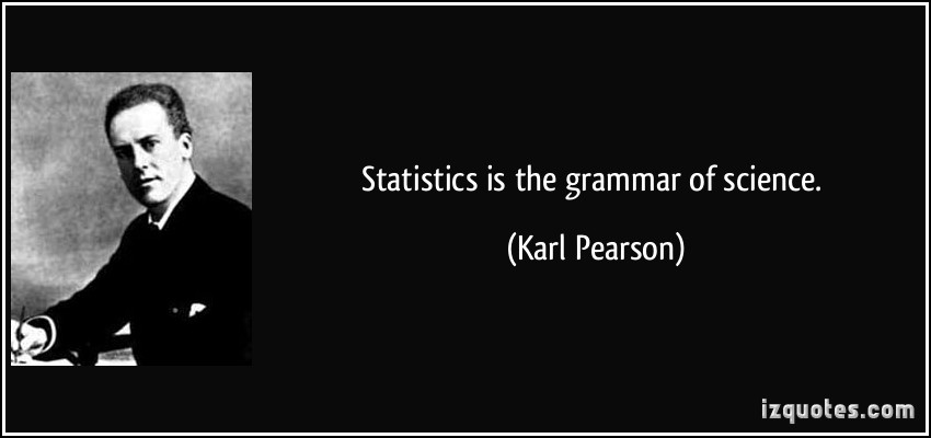 - Measures the strength of the linear relationship between two quantitative variables. - Does not completely characterize their relationship. --- #### Pearson's Correlation Coefficient $$ cor(x,y) = \frac{\sum_{i=1}^N (x_i-\mu_x)(y_i-\mu_y)}{N *\sigma_x \sigma_y} $$ <!--https://github.com/EvaMaeRey/statistics/blob/master/difference_in_difference.Rmd--> <!-- --> --- #### Covariance: Mean `\(x\)` $$ cov(x,y) = \frac{\sum_{i=1}^N (x_i-\mu_x)(y_i-\mu_y)}{N} $$ <!-- --> --- #### Covariance: Mean `\(y\)` $$ cov(x,y) = \frac{\sum_{i=1}^N (x_i-\mu_x)(y_i-\mu_y)}{N} $$ <!-- --> --- #### Covariance: differences `\(x\)` $$ cov(x,y) = \frac{\sum_{i=1}^N (x_i-\mu_x)(y_i-\mu_y)}{N} $$ <!-- --> --- #### Covariance: Differences `\(y\)` $$ cov(x,y) = \frac{\sum_{i=1}^N (x_i-\mu_x)(y_i-\mu_y)}{N} $$ <!-- --> --- #### Covariance: Multiply differences $$ cov(x,y) = \frac{\sum_{i=1}^N (x_i-\mu_x)(y_i-\mu_y)}{N} $$ 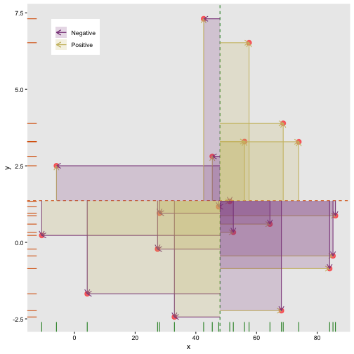<!-- --> --- #### Covariance: take average rectangle $$ cov(x,y) = \frac{\sum_{i=1}^N (x_i-\mu_x)(y_i-\mu_y)}{N} $$ <!-- --> --- .pull-left[ ### Covariance $$ cov(x,y) = \frac{\sum_{i=1}^N (x_i-\mu_x)(y_i-\mu_y)}{N} $$ $$ cor(x,y) = \frac{\sum_{i=1}^N (x_i-\mu_x)(y_i-\mu_y)}{N *\sigma_x \sigma_y} $$ `$$cor(x, y) = \frac{cov(x, y)}{\sigma_x \sigma_y}$$` ] .pull-right[ 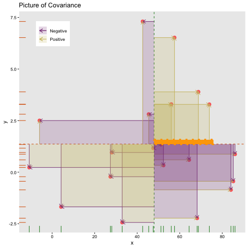<!-- --> ] --- # Variance and Standard Deviations $$ \sigma^2 = \frac{\sum_{i=1}^N (x_i-\mu_x)^2}{N} $$ $$ \sigma = \sqrt\frac{\sum_{i=1}^N (x_i-\mu_x)^2}{N} $$ --- # Variance .pull-left[ $$ \sigma^2 = \frac{\sum_{i=1}^N (x_i-\mu_x)^2}{N} $$ ] .pull-right[ 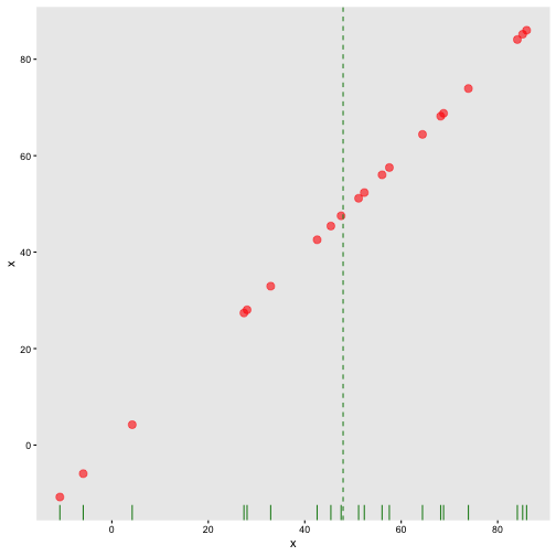<!-- --> ] --- # Variance .pull-left[ $$ \sigma^2 = \frac{\sum_{i=1}^N (x_i-\mu_x)^2}{N} $$ ] .pull-right[ 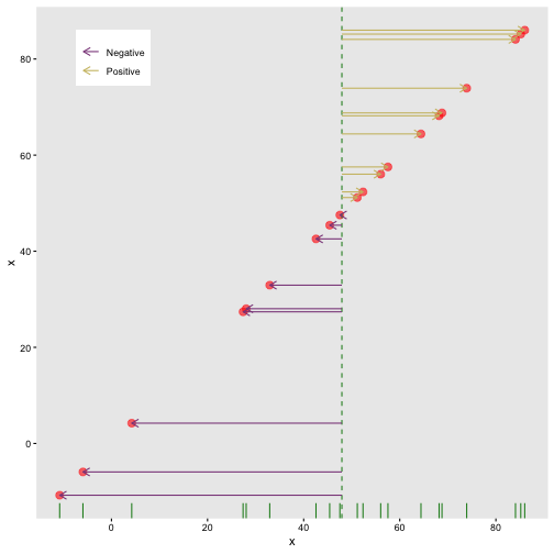<!-- --> ] --- ## Correlation: Beware $$ cor(x,y) = \frac{\sum_{i=1}^N (x_i-\mu_x)(y_i-\mu_y)}{N *\sigma_x \sigma_y} $$ $$ cor(x,y) = \frac{\sum_{i=1}^n (x_i-\bar{x})(y_i-\bar{y})}{(n-1) *S_x S_y} $$ --- ## Pearson's correlation coefficient - returns a value of between -1 and +1. A -1 means there is a strong negative correlation and +1 means that there is a strong positive correlation. - is very sensitive to outliers. .pull-left[ 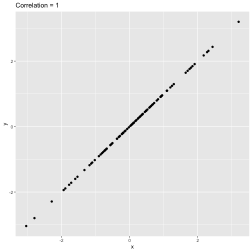<!-- --> ] .pull-right[ 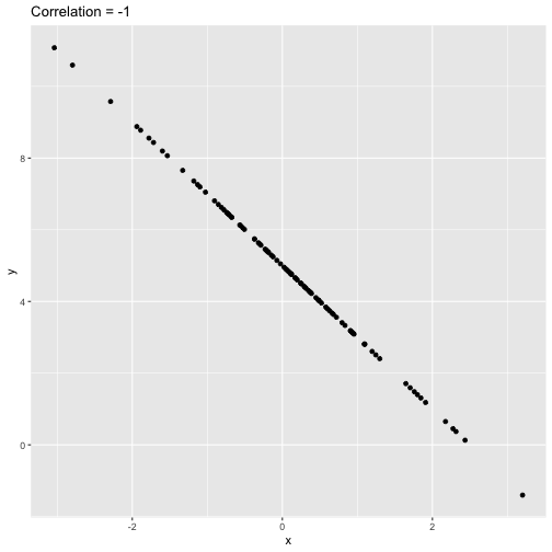<!-- --> ] --- ## Pearson's correlation coefficient (cont.) ```r set.seed(2020) x <- rnorm(100) y <- rnorm(100) df <- data.frame(x=x, y=y) ggplot(df, aes(x=x, y=y)) + geom_point()+xlab("x") + ylab("y") + ggtitle("Correlation = -0.03") + coord_equal() ``` 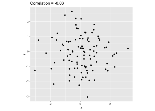<!-- --> --- ## Pearson's correlation coefficient (cont.) ```r set.seed(2020) x <- seq(-2, 2, length.out = 20) y <- 5*x^2 df <- data.frame(x=x, y=y) ggplot(df, aes(x=x, y=y)) + geom_point()+xlab("x") + ylab("y") + ggtitle("Correlation = ---") ``` 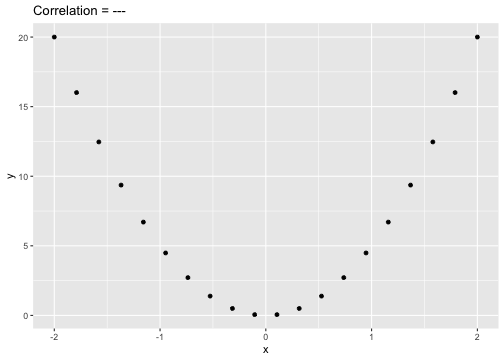<!-- --> --- ## Pearson's correlation coefficient (cont.) ```r cor(x, y) ``` ``` [1] -1.70372e-16 ``` ```r ggplot(df, aes(x=x, y=y)) + geom_point()+xlab("x") + ylab("y") + ggtitle("Correlation = 0.000") ``` 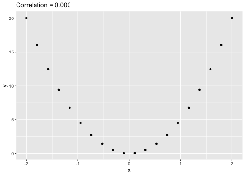<!-- --> --- ```r anscombe ``` ``` x1 x2 x3 x4 y1 y2 y3 y4 1 10 10 10 8 8.04 9.14 7.46 6.58 2 8 8 8 8 6.95 8.14 6.77 5.76 3 13 13 13 8 7.58 8.74 12.74 7.71 4 9 9 9 8 8.81 8.77 7.11 8.84 5 11 11 11 8 8.33 9.26 7.81 8.47 6 14 14 14 8 9.96 8.10 8.84 7.04 7 6 6 6 8 7.24 6.13 6.08 5.25 8 4 4 4 19 4.26 3.10 5.39 12.50 9 12 12 12 8 10.84 9.13 8.15 5.56 10 7 7 7 8 4.82 7.26 6.42 7.91 11 5 5 5 8 5.68 4.74 5.73 6.89 ``` --- ```r x <- c(anscombe$x1, anscombe$x2, anscombe$x3, anscombe$x4) y <- c(anscombe$y1, anscombe$y2, anscombe$y2, anscombe$y4) z <- as.factor(rep(1:4, each=11)) df <- data.frame(x=x, y=y, z=z) ggplot(df,aes(x=x,y=y,group=z))+geom_point(aes(col=z))+facet_wrap(~z) ``` 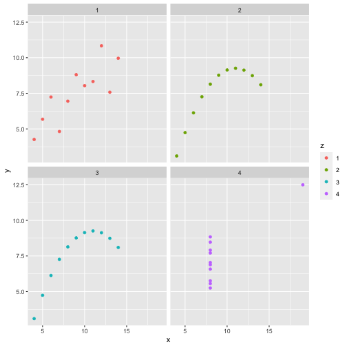<!-- --> --- .pull-left[ ```r cor(anscombe$x1, anscombe$y1) ``` ``` [1] 0.8164205 ``` ```r mean(anscombe$x1) ``` ``` [1] 9 ``` ```r mean(anscombe$y1) ``` ``` [1] 7.500909 ``` ```r cor(anscombe$x2, anscombe$y2) ``` ``` [1] 0.8162365 ``` ```r mean(anscombe$x2) ``` ``` [1] 9 ``` ```r mean(anscombe$y2) ``` ``` [1] 7.500909 ``` ] .pull-right[ ```r cor(anscombe$x3, anscombe$y3) ``` ``` [1] 0.8162867 ``` ```r mean(anscombe$x3) ``` ``` [1] 9 ``` ```r mean(anscombe$y3) ``` ``` [1] 7.5 ``` ```r cor(anscombe$x4, anscombe$y4) ``` ``` [1] 0.8165214 ``` ```r mean(anscombe$x4) ``` ``` [1] 9 ``` ```r mean(anscombe$y4) ``` ``` [1] 7.500909 ``` ] --- Anscombe's quartet ```r x <- c(anscombe$x1, anscombe$x2, anscombe$x3, anscombe$x4) y <- c(anscombe$y1, anscombe$y2, anscombe$y2, anscombe$y4) z <- as.factor(rep(1:4, each=11)) df <- data.frame(x=x, y=y, z=z) ggplot(df,aes(x=x,y=y,group=z))+geom_point(aes(col=z))+facet_wrap(~z) ``` 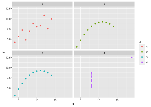<!-- --> All four sets are identical when examined using simple summary statistics but vary considerably when grouped. --- background-image: url('samestat_differentdata.png') background-position: center background-size: contain ---  Acknowledgement: Justin Matejke and George Fitzmaurice, Autodesk Research, Canada --- ## Regression Analysis ### Functional relationship between two variables <!-- --> --- ### Functional relationship between two variables <!-- --> --- ### Functional relationship between two variables <!-- --> --- ### Functional relationship between two variables <!-- --> --- ## For anyone who's interested in learning R programming Install R and R studio [Help is here](https://r4fun.netlify.app/blog/topic1/) --- ## Simple Linear Regression **Simple** - single regressor **Linear** - regression parameters enter in a linear fashion. --- ## Terminologies - Response variable: dependent variable - Explanatory variables: independent variables, predictors, regressor variables, features (in Machine Learning) - Parameter - Statistic - Estimator - Estimate [Read my blogpost](https://thiyanga.netlify.app/post/statterms1/) --- class: center, middle All rights reserved by [Dr. Thiyanga S. Talagala](https://thiyanga.netlify.app/) Acknowledgement Gina Reynolds, University of Denver.