class: center, middle, inverse, title-slide .title[ # EES 211 2.0 Data Analysis and Modeling ] .subtitle[ ## (Department of Physics, USJ) ] .author[ ### Dr Thiyanga Talagala ] .author[ ### Department of Statistics, University of Sri Jayewardenepura ] --- class: middle, left <style type="text/css"> .remark-slide-content { font-size: 45px; } </style> # What is Statistics? -- The science of collecting, analyzing, presenting, and interpreting data. --- class: center, middle # What is Statistics? The science of collecting, analyzing, presenting, and interpreting **data**. --- .pull-left[ 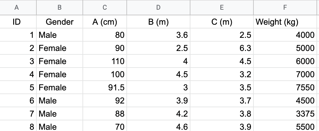 ] --- .pull-left[  ] .pull-right[ 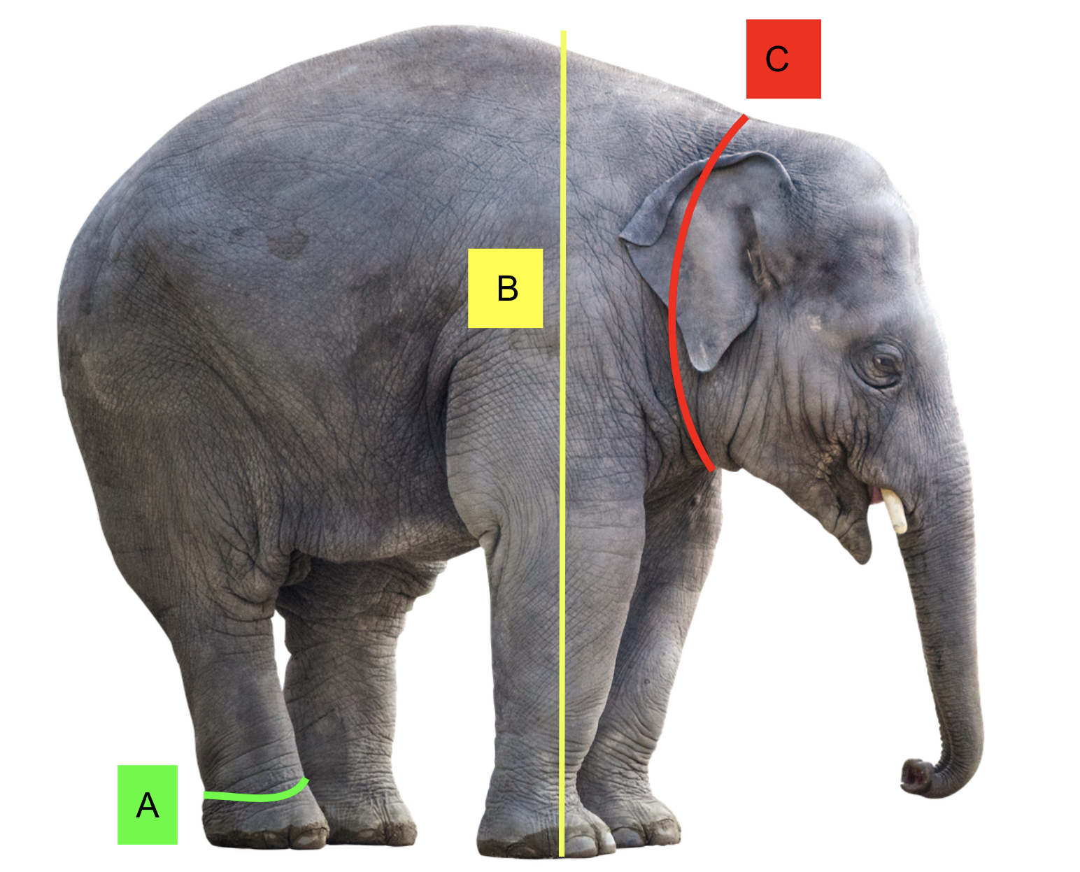 ] --- .pull-left[ **Tabular data**  ] .pull-right[ ] --- background-image: url(i4.png) background-size: contain --- .pull-left[ Tabular data  ] .pull-right[ **Image data**  ] --- .pull-left[ Tabular data  **Audio data**  ] .pull-right[ Image data  ] --- .pull-left[ Tabular data  Audio data  ] .pull-right[ Image data  **Video data** <iframe width="560" height="315" src="https://www.youtube.com/embed/398Zcag0Pw8" title="YouTube video player" frameborder="0" allow="accelerometer; autoplay; clipboard-write; encrypted-media; gyroscope; picture-in-picture" allowfullscreen></iframe> ] --- class: center, middle # What is Statistics? The science of **collecting**, analyzing, presenting, and interpreting **data**. --- class: center, middle # What is Statistics? The science of collecting, **analyzing**, presenting, and interpreting **data**. --- background-image: url(orange.jpeg) background-size: cover # Data analysis --- .pull-left[ ``` ID Gender A B C Weight 1 1 Male 80.0 3.6 2.5 4000 2 2 Female 90.0 2.5 6.3 5000 3 3 Female 110.0 4.0 4.5 6000 4 4 Female 100.0 4.5 3.2 7000 5 5 Female 91.5 3.0 3.5 7550 6 6 Male 92.0 3.9 3.7 4500 7 7 Male 88.0 4.2 3.8 3375 8 8 Male 70.0 4.6 3.9 5500 9 9 Female 100.5 2.9 1.2 2975 10 10 Female 99.8 3.7 4.2 3784 11 11 Female 101.5 2.7 2.2 2766 12 12 Female 99.2 5.1 4.4 5196 13 13 Female 99.6 3.8 3.9 3928 14 14 Female 99.1 2.7 3.1 2779 15 15 Female 99.8 4.0 4.8 4086 16 16 Female 100.4 4.2 2.8 4338 17 17 Female 99.3 4.1 2.9 4175 18 18 Female 100.8 3.2 2.5 3295 19 19 Female 98.8 5.0 2.8 5111 20 20 Female 99.0 3.9 4.4 3990 21 21 Female 101.4 2.9 3.9 2978 22 22 Female 99.0 1.3 4.5 1387 23 23 Female 100.4 4.6 3.1 4726 24 24 Female 99.6 3.5 3.9 3556 25 25 Female 100.4 3.5 3.7 3584 26 26 Female 101.7 4.4 2.1 4546 27 27 Female 101.6 4.3 5.3 4421 28 28 Female 99.7 4.1 3.6 4193 29 29 Female 97.7 4.4 4.3 4520 30 30 Female 102.5 4.3 4.5 4381 31 31 Female 100.7 3.6 3.4 3674 32 32 Female 100.5 1.5 3.2 1610 33 33 Female 100.0 4.1 4.4 4220 34 34 Female 100.5 3.4 2.5 3544 35 35 Female 99.8 3.3 5.5 3445 36 36 Female 100.4 2.0 3.1 2129 37 37 Female 99.6 3.0 5.2 3121 38 38 Female 98.6 3.9 5.0 4019 39 39 Female 101.0 4.9 3.6 4958 40 40 Female 101.5 3.4 4.1 3497 41 41 Female 99.7 3.9 2.5 3988 42 42 Female 98.7 3.4 3.8 3547 43 43 Female 100.6 2.1 4.5 2223 44 44 Female 100.0 3.1 3.6 3185 45 45 Female 98.3 3.1 3.0 3205 46 46 Female 100.0 3.4 2.8 3540 47 47 Female 99.4 4.6 3.5 4700 48 48 Female 99.7 4.3 4.6 4363 49 49 Female 98.8 3.3 3.0 3436 50 50 Female 101.8 3.2 3.4 3345 51 51 Female 99.7 4.2 2.2 4297 52 52 Female 98.4 4.1 4.0 4155 53 53 Female 100.2 2.8 4.8 2911 54 54 Female 100.3 2.8 5.0 2892 55 55 Male 99.0 3.4 4.3 5146 56 56 Male 97.1 3.8 1.6 5753 57 57 Male 99.4 2.9 4.0 4430 58 58 Male 100.6 3.9 4.0 5923 59 59 Male 99.9 3.4 3.1 5195 60 60 Male 99.9 2.4 3.7 3681 61 61 Male 100.6 3.3 2.6 5111 62 62 Male 98.8 1.9 4.2 2905 63 63 Male 101.1 4.4 3.2 6752 64 64 Male 100.0 5.0 1.9 7571 65 65 Male 100.7 2.6 3.1 4048 66 66 Male 101.0 2.0 4.9 3032 67 67 Male 100.2 3.6 3.2 5455 68 68 Male 99.1 2.9 4.2 4397 69 69 Male 101.2 5.4 4.4 8202 70 70 Male 98.0 3.0 3.5 4540 71 71 Male 99.5 3.7 3.1 5633 72 72 Male 99.7 3.0 3.0 4641 73 73 Male 99.8 2.3 4.2 3486 74 74 Male 101.0 3.2 2.4 4883 75 75 Male 100.1 1.2 3.7 1891 76 76 Male 100.4 4.5 3.2 6800 77 77 Male 99.9 3.2 1.2 4830 78 78 Male 99.8 5.2 2.1 7859 79 79 Male 100.7 3.5 4.4 5314 80 80 Male 101.1 2.3 3.3 3536 81 81 Male 97.6 3.6 4.3 5515 82 82 Male 100.6 2.1 5.4 3201 83 83 Male 100.4 1.7 5.0 2719 84 84 Male 99.6 3.3 4.2 5036 85 85 Male 101.0 2.6 3.9 3935 86 86 Male 99.6 3.0 3.3 4602 87 87 Male 99.7 3.1 5.1 4714 88 88 Male 100.9 2.4 4.1 3716 89 89 Male 101.7 2.4 2.3 3747 90 90 Male 100.3 2.9 3.3 4397 91 91 Male 99.6 4.2 1.6 6367 92 92 Male 98.8 1.5 3.3 2315 93 93 Male 99.7 3.6 0.9 5492 94 94 Male 99.1 3.3 4.8 5102 95 95 Male 99.7 4.1 2.9 6196 96 96 Male 100.4 2.7 3.1 4145 97 97 Male 99.1 3.4 3.3 5154 98 98 Male 102.6 3.3 4.1 5002 99 99 Male 100.2 2.5 4.2 3786 100 100 Male 101.1 4.2 4.1 6410 ``` ] -- .pull-right[ <img src="ees211_1_files/figure-html/unnamed-chunk-2-1.png" width="100%" /> ] --- .pull-left[ ``` ID Gender A B C Weight 1 1 Male 80.0 3.6 2.5 4000 2 2 Female 90.0 2.5 6.3 5000 3 3 Female 110.0 4.0 4.5 6000 4 4 Female 100.0 4.5 3.2 7000 5 5 Female 91.5 3.0 3.5 7550 6 6 Male 92.0 3.9 3.7 4500 7 7 Male 88.0 4.2 3.8 3375 8 8 Male 70.0 4.6 3.9 5500 9 9 Female 100.5 2.9 1.2 2975 10 10 Female 99.8 3.7 4.2 3784 11 11 Female 101.5 2.7 2.2 2766 12 12 Female 99.2 5.1 4.4 5196 13 13 Female 99.6 3.8 3.9 3928 14 14 Female 99.1 2.7 3.1 2779 15 15 Female 99.8 4.0 4.8 4086 16 16 Female 100.4 4.2 2.8 4338 17 17 Female 99.3 4.1 2.9 4175 18 18 Female 100.8 3.2 2.5 3295 19 19 Female 98.8 5.0 2.8 5111 20 20 Female 99.0 3.9 4.4 3990 21 21 Female 101.4 2.9 3.9 2978 22 22 Female 99.0 1.3 4.5 1387 23 23 Female 100.4 4.6 3.1 4726 24 24 Female 99.6 3.5 3.9 3556 25 25 Female 100.4 3.5 3.7 3584 26 26 Female 101.7 4.4 2.1 4546 27 27 Female 101.6 4.3 5.3 4421 28 28 Female 99.7 4.1 3.6 4193 29 29 Female 97.7 4.4 4.3 4520 30 30 Female 102.5 4.3 4.5 4381 31 31 Female 100.7 3.6 3.4 3674 32 32 Female 100.5 1.5 3.2 1610 33 33 Female 100.0 4.1 4.4 4220 34 34 Female 100.5 3.4 2.5 3544 35 35 Female 99.8 3.3 5.5 3445 36 36 Female 100.4 2.0 3.1 2129 37 37 Female 99.6 3.0 5.2 3121 38 38 Female 98.6 3.9 5.0 4019 39 39 Female 101.0 4.9 3.6 4958 40 40 Female 101.5 3.4 4.1 3497 41 41 Female 99.7 3.9 2.5 3988 42 42 Female 98.7 3.4 3.8 3547 43 43 Female 100.6 2.1 4.5 2223 44 44 Female 100.0 3.1 3.6 3185 45 45 Female 98.3 3.1 3.0 3205 46 46 Female 100.0 3.4 2.8 3540 47 47 Female 99.4 4.6 3.5 4700 48 48 Female 99.7 4.3 4.6 4363 49 49 Female 98.8 3.3 3.0 3436 50 50 Female 101.8 3.2 3.4 3345 51 51 Female 99.7 4.2 2.2 4297 52 52 Female 98.4 4.1 4.0 4155 53 53 Female 100.2 2.8 4.8 2911 54 54 Female 100.3 2.8 5.0 2892 55 55 Male 99.0 3.4 4.3 5146 56 56 Male 97.1 3.8 1.6 5753 57 57 Male 99.4 2.9 4.0 4430 58 58 Male 100.6 3.9 4.0 5923 59 59 Male 99.9 3.4 3.1 5195 60 60 Male 99.9 2.4 3.7 3681 61 61 Male 100.6 3.3 2.6 5111 62 62 Male 98.8 1.9 4.2 2905 63 63 Male 101.1 4.4 3.2 6752 64 64 Male 100.0 5.0 1.9 7571 65 65 Male 100.7 2.6 3.1 4048 66 66 Male 101.0 2.0 4.9 3032 67 67 Male 100.2 3.6 3.2 5455 68 68 Male 99.1 2.9 4.2 4397 69 69 Male 101.2 5.4 4.4 8202 70 70 Male 98.0 3.0 3.5 4540 71 71 Male 99.5 3.7 3.1 5633 72 72 Male 99.7 3.0 3.0 4641 73 73 Male 99.8 2.3 4.2 3486 74 74 Male 101.0 3.2 2.4 4883 75 75 Male 100.1 1.2 3.7 1891 76 76 Male 100.4 4.5 3.2 6800 77 77 Male 99.9 3.2 1.2 4830 78 78 Male 99.8 5.2 2.1 7859 79 79 Male 100.7 3.5 4.4 5314 80 80 Male 101.1 2.3 3.3 3536 81 81 Male 97.6 3.6 4.3 5515 82 82 Male 100.6 2.1 5.4 3201 83 83 Male 100.4 1.7 5.0 2719 84 84 Male 99.6 3.3 4.2 5036 85 85 Male 101.0 2.6 3.9 3935 86 86 Male 99.6 3.0 3.3 4602 87 87 Male 99.7 3.1 5.1 4714 88 88 Male 100.9 2.4 4.1 3716 89 89 Male 101.7 2.4 2.3 3747 90 90 Male 100.3 2.9 3.3 4397 91 91 Male 99.6 4.2 1.6 6367 92 92 Male 98.8 1.5 3.3 2315 93 93 Male 99.7 3.6 0.9 5492 94 94 Male 99.1 3.3 4.8 5102 95 95 Male 99.7 4.1 2.9 6196 96 96 Male 100.4 2.7 3.1 4145 97 97 Male 99.1 3.4 3.3 5154 98 98 Male 102.6 3.3 4.1 5002 99 99 Male 100.2 2.5 4.2 3786 100 100 Male 101.1 4.2 4.1 6410 ``` ] .pull-right[ <img src="ees211_1_files/figure-html/unnamed-chunk-4-1.png" width="100%" /> ] --- .pull-left[ ``` ID Gender A B C Weight 1 1 Male 80.0 3.6 2.5 4000 2 2 Female 90.0 2.5 6.3 5000 3 3 Female 110.0 4.0 4.5 6000 4 4 Female 100.0 4.5 3.2 7000 5 5 Female 91.5 3.0 3.5 7550 6 6 Male 92.0 3.9 3.7 4500 7 7 Male 88.0 4.2 3.8 3375 8 8 Male 70.0 4.6 3.9 5500 9 9 Female 100.5 2.9 1.2 2975 10 10 Female 99.8 3.7 4.2 3784 11 11 Female 101.5 2.7 2.2 2766 12 12 Female 99.2 5.1 4.4 5196 13 13 Female 99.6 3.8 3.9 3928 14 14 Female 99.1 2.7 3.1 2779 15 15 Female 99.8 4.0 4.8 4086 16 16 Female 100.4 4.2 2.8 4338 17 17 Female 99.3 4.1 2.9 4175 18 18 Female 100.8 3.2 2.5 3295 19 19 Female 98.8 5.0 2.8 5111 20 20 Female 99.0 3.9 4.4 3990 21 21 Female 101.4 2.9 3.9 2978 22 22 Female 99.0 1.3 4.5 1387 23 23 Female 100.4 4.6 3.1 4726 24 24 Female 99.6 3.5 3.9 3556 25 25 Female 100.4 3.5 3.7 3584 26 26 Female 101.7 4.4 2.1 4546 27 27 Female 101.6 4.3 5.3 4421 28 28 Female 99.7 4.1 3.6 4193 29 29 Female 97.7 4.4 4.3 4520 30 30 Female 102.5 4.3 4.5 4381 31 31 Female 100.7 3.6 3.4 3674 32 32 Female 100.5 1.5 3.2 1610 33 33 Female 100.0 4.1 4.4 4220 34 34 Female 100.5 3.4 2.5 3544 35 35 Female 99.8 3.3 5.5 3445 36 36 Female 100.4 2.0 3.1 2129 37 37 Female 99.6 3.0 5.2 3121 38 38 Female 98.6 3.9 5.0 4019 39 39 Female 101.0 4.9 3.6 4958 40 40 Female 101.5 3.4 4.1 3497 41 41 Female 99.7 3.9 2.5 3988 42 42 Female 98.7 3.4 3.8 3547 43 43 Female 100.6 2.1 4.5 2223 44 44 Female 100.0 3.1 3.6 3185 45 45 Female 98.3 3.1 3.0 3205 46 46 Female 100.0 3.4 2.8 3540 47 47 Female 99.4 4.6 3.5 4700 48 48 Female 99.7 4.3 4.6 4363 49 49 Female 98.8 3.3 3.0 3436 50 50 Female 101.8 3.2 3.4 3345 51 51 Female 99.7 4.2 2.2 4297 52 52 Female 98.4 4.1 4.0 4155 53 53 Female 100.2 2.8 4.8 2911 54 54 Female 100.3 2.8 5.0 2892 55 55 Male 99.0 3.4 4.3 5146 56 56 Male 97.1 3.8 1.6 5753 57 57 Male 99.4 2.9 4.0 4430 58 58 Male 100.6 3.9 4.0 5923 59 59 Male 99.9 3.4 3.1 5195 60 60 Male 99.9 2.4 3.7 3681 61 61 Male 100.6 3.3 2.6 5111 62 62 Male 98.8 1.9 4.2 2905 63 63 Male 101.1 4.4 3.2 6752 64 64 Male 100.0 5.0 1.9 7571 65 65 Male 100.7 2.6 3.1 4048 66 66 Male 101.0 2.0 4.9 3032 67 67 Male 100.2 3.6 3.2 5455 68 68 Male 99.1 2.9 4.2 4397 69 69 Male 101.2 5.4 4.4 8202 70 70 Male 98.0 3.0 3.5 4540 71 71 Male 99.5 3.7 3.1 5633 72 72 Male 99.7 3.0 3.0 4641 73 73 Male 99.8 2.3 4.2 3486 74 74 Male 101.0 3.2 2.4 4883 75 75 Male 100.1 1.2 3.7 1891 76 76 Male 100.4 4.5 3.2 6800 77 77 Male 99.9 3.2 1.2 4830 78 78 Male 99.8 5.2 2.1 7859 79 79 Male 100.7 3.5 4.4 5314 80 80 Male 101.1 2.3 3.3 3536 81 81 Male 97.6 3.6 4.3 5515 82 82 Male 100.6 2.1 5.4 3201 83 83 Male 100.4 1.7 5.0 2719 84 84 Male 99.6 3.3 4.2 5036 85 85 Male 101.0 2.6 3.9 3935 86 86 Male 99.6 3.0 3.3 4602 87 87 Male 99.7 3.1 5.1 4714 88 88 Male 100.9 2.4 4.1 3716 89 89 Male 101.7 2.4 2.3 3747 90 90 Male 100.3 2.9 3.3 4397 91 91 Male 99.6 4.2 1.6 6367 92 92 Male 98.8 1.5 3.3 2315 93 93 Male 99.7 3.6 0.9 5492 94 94 Male 99.1 3.3 4.8 5102 95 95 Male 99.7 4.1 2.9 6196 96 96 Male 100.4 2.7 3.1 4145 97 97 Male 99.1 3.4 3.3 5154 98 98 Male 102.6 3.3 4.1 5002 99 99 Male 100.2 2.5 4.2 3786 100 100 Male 101.1 4.2 4.1 6410 ``` ] .pull-right[ <div id="htmlwidget-91721eeb47d605788ab2" style="width:100%;height:504px;" class="plotly html-widget"></div> <script type="application/json" data-for="htmlwidget-91721eeb47d605788ab2">{"x":{"data":[{"x":[2.5,4,4.5,3,2.9,3.7,2.7,5.1,3.8,2.7,4,4.2,4.1,3.2,5,3.9,2.9,1.3,4.6,3.5,3.5,4.4,4.3,4.1,4.4,4.3,3.6,1.5,4.1,3.4,3.3,2,3,3.9,4.9,3.4,3.9,3.4,2.1,3.1,3.1,3.4,4.6,4.3,3.3,3.2,4.2,4.1,2.8,2.8],"y":[5000,6000,7000,7550,2975,3784,2766,5196,3928,2779,4086,4338,4175,3295,5111,3990,2978,1387,4726,3556,3584,4546,4421,4193,4520,4381,3674,1610,4220,3544,3445,2129,3121,4019,4958,3497,3988,3547,2223,3185,3205,3540,4700,4363,3436,3345,4297,4155,2911,2892],"text":["B: 2.5<br />Weight: 5000<br />Gender: Female","B: 4.0<br />Weight: 6000<br />Gender: Female","B: 4.5<br />Weight: 7000<br />Gender: Female","B: 3.0<br />Weight: 7550<br />Gender: Female","B: 2.9<br />Weight: 2975<br />Gender: Female","B: 3.7<br />Weight: 3784<br />Gender: Female","B: 2.7<br />Weight: 2766<br />Gender: Female","B: 5.1<br />Weight: 5196<br />Gender: Female","B: 3.8<br />Weight: 3928<br />Gender: Female","B: 2.7<br />Weight: 2779<br />Gender: Female","B: 4.0<br />Weight: 4086<br />Gender: Female","B: 4.2<br />Weight: 4338<br />Gender: Female","B: 4.1<br />Weight: 4175<br />Gender: Female","B: 3.2<br />Weight: 3295<br />Gender: Female","B: 5.0<br />Weight: 5111<br />Gender: Female","B: 3.9<br />Weight: 3990<br />Gender: Female","B: 2.9<br />Weight: 2978<br />Gender: Female","B: 1.3<br />Weight: 1387<br />Gender: Female","B: 4.6<br />Weight: 4726<br />Gender: Female","B: 3.5<br />Weight: 3556<br />Gender: Female","B: 3.5<br />Weight: 3584<br />Gender: Female","B: 4.4<br />Weight: 4546<br />Gender: Female","B: 4.3<br />Weight: 4421<br />Gender: Female","B: 4.1<br />Weight: 4193<br />Gender: Female","B: 4.4<br />Weight: 4520<br />Gender: Female","B: 4.3<br />Weight: 4381<br />Gender: Female","B: 3.6<br />Weight: 3674<br />Gender: Female","B: 1.5<br />Weight: 1610<br />Gender: Female","B: 4.1<br />Weight: 4220<br />Gender: Female","B: 3.4<br />Weight: 3544<br />Gender: Female","B: 3.3<br />Weight: 3445<br />Gender: Female","B: 2.0<br />Weight: 2129<br />Gender: Female","B: 3.0<br />Weight: 3121<br />Gender: Female","B: 3.9<br />Weight: 4019<br />Gender: Female","B: 4.9<br />Weight: 4958<br />Gender: Female","B: 3.4<br />Weight: 3497<br />Gender: Female","B: 3.9<br />Weight: 3988<br />Gender: Female","B: 3.4<br />Weight: 3547<br />Gender: Female","B: 2.1<br />Weight: 2223<br />Gender: Female","B: 3.1<br />Weight: 3185<br />Gender: Female","B: 3.1<br />Weight: 3205<br />Gender: Female","B: 3.4<br />Weight: 3540<br />Gender: Female","B: 4.6<br />Weight: 4700<br />Gender: Female","B: 4.3<br />Weight: 4363<br />Gender: Female","B: 3.3<br />Weight: 3436<br />Gender: Female","B: 3.2<br />Weight: 3345<br />Gender: Female","B: 4.2<br />Weight: 4297<br />Gender: Female","B: 4.1<br />Weight: 4155<br />Gender: Female","B: 2.8<br />Weight: 2911<br />Gender: Female","B: 2.8<br />Weight: 2892<br />Gender: Female"],"type":"scatter","mode":"markers","marker":{"autocolorscale":false,"color":"rgba(231,41,138,1)","opacity":1,"size":5.66929133858268,"symbol":"circle","line":{"width":1.88976377952756,"color":"rgba(231,41,138,1)"}},"hoveron":"points","name":"Female","legendgroup":"Female","showlegend":true,"xaxis":"x","yaxis":"y","hoverinfo":"text","frame":null},{"x":[3.6,3.9,4.2,4.6,3.4,3.8,2.9,3.9,3.4,2.4,3.3,1.9,4.4,5,2.6,2,3.6,2.9,5.4,3,3.7,3,2.3,3.2,1.2,4.5,3.2,5.2,3.5,2.3,3.6,2.1,1.7,3.3,2.6,3,3.1,2.4,2.4,2.9,4.2,1.5,3.6,3.3,4.1,2.7,3.4,3.3,2.5,4.2],"y":[4000,4500,3375,5500,5146,5753,4430,5923,5195,3681,5111,2905,6752,7571,4048,3032,5455,4397,8202,4540,5633,4641,3486,4883,1891,6800,4830,7859,5314,3536,5515,3201,2719,5036,3935,4602,4714,3716,3747,4397,6367,2315,5492,5102,6196,4145,5154,5002,3786,6410],"text":["B: 3.6<br />Weight: 4000<br />Gender: Male","B: 3.9<br />Weight: 4500<br />Gender: Male","B: 4.2<br />Weight: 3375<br />Gender: Male","B: 4.6<br />Weight: 5500<br />Gender: Male","B: 3.4<br />Weight: 5146<br />Gender: Male","B: 3.8<br />Weight: 5753<br />Gender: Male","B: 2.9<br />Weight: 4430<br />Gender: Male","B: 3.9<br />Weight: 5923<br />Gender: Male","B: 3.4<br />Weight: 5195<br />Gender: Male","B: 2.4<br />Weight: 3681<br />Gender: Male","B: 3.3<br />Weight: 5111<br />Gender: Male","B: 1.9<br />Weight: 2905<br />Gender: Male","B: 4.4<br />Weight: 6752<br />Gender: Male","B: 5.0<br />Weight: 7571<br />Gender: Male","B: 2.6<br />Weight: 4048<br />Gender: Male","B: 2.0<br />Weight: 3032<br />Gender: Male","B: 3.6<br />Weight: 5455<br />Gender: Male","B: 2.9<br />Weight: 4397<br />Gender: Male","B: 5.4<br />Weight: 8202<br />Gender: Male","B: 3.0<br />Weight: 4540<br />Gender: Male","B: 3.7<br />Weight: 5633<br />Gender: Male","B: 3.0<br />Weight: 4641<br />Gender: Male","B: 2.3<br />Weight: 3486<br />Gender: Male","B: 3.2<br />Weight: 4883<br />Gender: Male","B: 1.2<br />Weight: 1891<br />Gender: Male","B: 4.5<br />Weight: 6800<br />Gender: Male","B: 3.2<br />Weight: 4830<br />Gender: Male","B: 5.2<br />Weight: 7859<br />Gender: Male","B: 3.5<br />Weight: 5314<br />Gender: Male","B: 2.3<br />Weight: 3536<br />Gender: Male","B: 3.6<br />Weight: 5515<br />Gender: Male","B: 2.1<br />Weight: 3201<br />Gender: Male","B: 1.7<br />Weight: 2719<br />Gender: Male","B: 3.3<br />Weight: 5036<br />Gender: Male","B: 2.6<br />Weight: 3935<br />Gender: Male","B: 3.0<br />Weight: 4602<br />Gender: Male","B: 3.1<br />Weight: 4714<br />Gender: Male","B: 2.4<br />Weight: 3716<br />Gender: Male","B: 2.4<br />Weight: 3747<br />Gender: Male","B: 2.9<br />Weight: 4397<br />Gender: Male","B: 4.2<br />Weight: 6367<br />Gender: Male","B: 1.5<br />Weight: 2315<br />Gender: Male","B: 3.6<br />Weight: 5492<br />Gender: Male","B: 3.3<br />Weight: 5102<br />Gender: Male","B: 4.1<br />Weight: 6196<br />Gender: Male","B: 2.7<br />Weight: 4145<br />Gender: Male","B: 3.4<br />Weight: 5154<br />Gender: Male","B: 3.3<br />Weight: 5002<br />Gender: Male","B: 2.5<br />Weight: 3786<br />Gender: Male","B: 4.2<br />Weight: 6410<br />Gender: Male"],"type":"scatter","mode":"markers","marker":{"autocolorscale":false,"color":"rgba(27,158,119,1)","opacity":1,"size":5.66929133858268,"symbol":"circle","line":{"width":1.88976377952756,"color":"rgba(27,158,119,1)"}},"hoveron":"points","name":"Male","legendgroup":"Male","showlegend":true,"xaxis":"x","yaxis":"y","hoverinfo":"text","frame":null}],"layout":{"margin":{"t":40.8401826484018,"r":7.30593607305936,"b":37.2602739726027,"l":48.9497716894977},"plot_bgcolor":"rgba(235,235,235,1)","paper_bgcolor":"rgba(255,255,255,1)","font":{"color":"rgba(0,0,0,1)","family":"","size":14.6118721461187},"title":{"text":"Scatterplot of weight (kg) vs B (ft)","font":{"color":"rgba(0,0,0,1)","family":"","size":17.5342465753425},"x":0.5,"xref":"paper"},"xaxis":{"domain":[0,1],"automargin":true,"type":"linear","autorange":false,"range":[0.99,5.61],"tickmode":"array","ticktext":["1","2","3","4","5"],"tickvals":[1,2,3,4,5],"categoryorder":"array","categoryarray":["1","2","3","4","5"],"nticks":null,"ticks":"outside","tickcolor":"rgba(51,51,51,1)","ticklen":3.65296803652968,"tickwidth":0.66417600664176,"showticklabels":true,"tickfont":{"color":"rgba(77,77,77,1)","family":"","size":11.689497716895},"tickangle":-0,"showline":false,"linecolor":null,"linewidth":0,"showgrid":true,"gridcolor":"rgba(255,255,255,1)","gridwidth":0.66417600664176,"zeroline":false,"anchor":"y","title":{"text":"B (ft)","font":{"color":"rgba(0,0,0,1)","family":"","size":14.6118721461187}},"hoverformat":".2f"},"yaxis":{"domain":[0,1],"automargin":true,"type":"linear","autorange":false,"range":[1046.25,8542.75],"tickmode":"array","ticktext":["2000","4000","6000","8000"],"tickvals":[2000,4000,6000,8000],"categoryorder":"array","categoryarray":["2000","4000","6000","8000"],"nticks":null,"ticks":"outside","tickcolor":"rgba(51,51,51,1)","ticklen":3.65296803652968,"tickwidth":0.66417600664176,"showticklabels":true,"tickfont":{"color":"rgba(77,77,77,1)","family":"","size":11.689497716895},"tickangle":-0,"showline":false,"linecolor":null,"linewidth":0,"showgrid":true,"gridcolor":"rgba(255,255,255,1)","gridwidth":0.66417600664176,"zeroline":false,"anchor":"x","title":{"text":"Weight (kg)","font":{"color":"rgba(0,0,0,1)","family":"","size":14.6118721461187}},"hoverformat":".2f"},"shapes":[{"type":"rect","fillcolor":null,"line":{"color":null,"width":0,"linetype":[]},"yref":"paper","xref":"paper","x0":0,"x1":1,"y0":0,"y1":1}],"showlegend":true,"legend":{"bgcolor":"rgba(255,255,255,1)","bordercolor":"transparent","borderwidth":1.88976377952756,"font":{"color":"rgba(0,0,0,1)","family":"","size":11.689497716895},"title":{"text":"Gender","font":{"color":"rgba(0,0,0,1)","family":"","size":14.6118721461187}}},"hovermode":"closest","barmode":"relative"},"config":{"doubleClick":"reset","modeBarButtonsToAdd":["hoverclosest","hovercompare"],"showSendToCloud":false},"source":"A","attrs":{"4d14af79542":{"x":{},"y":{},"colour":{},"type":"scatter"}},"cur_data":"4d14af79542","visdat":{"4d14af79542":["function (y) ","x"]},"highlight":{"on":"plotly_click","persistent":false,"dynamic":false,"selectize":false,"opacityDim":0.2,"selected":{"opacity":1},"debounce":0},"shinyEvents":["plotly_hover","plotly_click","plotly_selected","plotly_relayout","plotly_brushed","plotly_brushing","plotly_clickannotation","plotly_doubleclick","plotly_deselect","plotly_afterplot","plotly_sunburstclick"],"base_url":"https://plot.ly"},"evals":[],"jsHooks":[]}</script> ] --- background-image: url(i7.png) background-size: cover --- class: center, middle # What is Statistics? The science of collecting, analyzing, **presenting, and interpreting** **data**. --- class: center, middle # Myth-busting Statistics -- Popular Myths (**false beliefs**) about statistics --- class: inverse, center, middle **Myth 1** **Statistics is a boring subject.** --- class: inverse, center, middle ~~**Myth 1**~~ **Statistics is a** ~~**boring subject**~~. # **Statistics is a** very interesting and useful subject with so many applications. --- background-image: url(i8.png) background-size: contain --- background-image: url(i9.jpeg) background-size: contain --- background-image: url(l2.png) background-size: contain --- background-image: url(l1.png) background-size: contain --- background-image: url(bp.jpg) background-size: contain --- background-image: url(s1.png) background-size: contain --- background-image: url(sydney.jpg) background-size: contain --- # Your Turn ## Assignment 1 Application of statistics in your field. Method of evaluation: 1 slide Time: 3 minutes Upload your video recording to the LMS Marks: 10 marks --- class: inverse, center, middle **Myth 2** **Statistics hasn't changed much in years. It is just the same old stuff.** --- class: inverse, center, middle ~~**Myth 2**~~ ~~**Statistics hasn't changed much in years. It is just the same old stuff.**~~ ## The field of statistics has evolved significantly over time. It has also become a main componenet of many other disciplines. --- # Ross Ihaka and Robert Gentleman .pull-left[ <img src="rr.jpg" width="100%" height="100%" /> ] .pull-right[ - Originators of the R programming language - R is a free software environment for statistical computing and graphics ] --- # Hadley Wickham: Chief Scientist at RStudio .pull-left[ <img src="HadleyWickham.png" width="100%" /> ] .pull-right[ - International COPSS Presidents' Award in 2019 for "influential work in statistical computing, visualisation, graphics, and data analysis" ] --- # Robert Tibshirani .pull-left[ <img src="Robert_tibshirani.png" width="100%" /> ] .pull-right[ - Professor in Statistics and Biomedical Data Science at Stanford University - Received the COPSS Presidents' Award in 1996 ] --- # Trevor Hastie .pull-left[ <img src="TrevorHastie.png" width="100%" /> ] .pull-right[ - Hastie is known for his contributions to applied statistics, especially in the field of machine learning, data mining, and bioinformatics. ] --- # Andrew Ng .pull-left[ <img src="Andrew_Ng.jpg" width="70%" /> ] .pull-right[ - Undergraduate degree with a triple major in computer science, **statistics**, and economics - Co-founded and led Google Brain, Coursera and deeplearning.ai ] --- background-image: url(f1.png) background-size: contain ## Data Science --- background-image: url(f2.png) background-size: contain ## Data Science --- background-image: url(f3.png) background-size: contain ## Data Science --- ## Statistics - Descriptive statistics/ Exploratory Data Analysis (EDA) > Use of graphical and numerical summaries to highlight the key features of data. - Inferential statistics > Techniques for drawing conclusions about a population by examining random samples --- ## Example Objective: Design a new chair for the university lecture halls Wants to identify right handed left handed count --- ## Population A population is a complete collection of individuals/ objects that we are interested in. ## Sample A sample is a subset of a population. --- ## Parameter A parameter is a descriptive measure(numerical value) of the population. Parameters are usually denoted by Greek letters. `\(\theta\)` - population proportion `\(\mu\)` - population mean --- ## Statistic A statistic is a descriptive measure of a sample. For example, sample mean, sample standard deviation, etc. We will talk about the notations under estimator and estimate. --- ## Variables **1. Qualitative/ Categorical** - Nominal, Ordinal **2. Quantitative/ Numerical** - Discrete, Continuous --- ## Your turn ```r data("mtcars") mtcars ``` ``` ## mpg cyl disp hp drat wt qsec vs am gear carb ## Mazda RX4 21.0 6 160.0 110 3.90 2.620 16.46 0 1 4 4 ## Mazda RX4 Wag 21.0 6 160.0 110 3.90 2.875 17.02 0 1 4 4 ## Datsun 710 22.8 4 108.0 93 3.85 2.320 18.61 1 1 4 1 ## Hornet 4 Drive 21.4 6 258.0 110 3.08 3.215 19.44 1 0 3 1 ## Hornet Sportabout 18.7 8 360.0 175 3.15 3.440 17.02 0 0 3 2 ## Valiant 18.1 6 225.0 105 2.76 3.460 20.22 1 0 3 1 ## Duster 360 14.3 8 360.0 245 3.21 3.570 15.84 0 0 3 4 ## Merc 240D 24.4 4 146.7 62 3.69 3.190 20.00 1 0 4 2 ## Merc 230 22.8 4 140.8 95 3.92 3.150 22.90 1 0 4 2 ## Merc 280 19.2 6 167.6 123 3.92 3.440 18.30 1 0 4 4 ## Merc 280C 17.8 6 167.6 123 3.92 3.440 18.90 1 0 4 4 ## Merc 450SE 16.4 8 275.8 180 3.07 4.070 17.40 0 0 3 3 ## Merc 450SL 17.3 8 275.8 180 3.07 3.730 17.60 0 0 3 3 ## Merc 450SLC 15.2 8 275.8 180 3.07 3.780 18.00 0 0 3 3 ## Cadillac Fleetwood 10.4 8 472.0 205 2.93 5.250 17.98 0 0 3 4 ## Lincoln Continental 10.4 8 460.0 215 3.00 5.424 17.82 0 0 3 4 ## Chrysler Imperial 14.7 8 440.0 230 3.23 5.345 17.42 0 0 3 4 ## Fiat 128 32.4 4 78.7 66 4.08 2.200 19.47 1 1 4 1 ## Honda Civic 30.4 4 75.7 52 4.93 1.615 18.52 1 1 4 2 ## Toyota Corolla 33.9 4 71.1 65 4.22 1.835 19.90 1 1 4 1 ## Toyota Corona 21.5 4 120.1 97 3.70 2.465 20.01 1 0 3 1 ## Dodge Challenger 15.5 8 318.0 150 2.76 3.520 16.87 0 0 3 2 ## AMC Javelin 15.2 8 304.0 150 3.15 3.435 17.30 0 0 3 2 ## Camaro Z28 13.3 8 350.0 245 3.73 3.840 15.41 0 0 3 4 ## Pontiac Firebird 19.2 8 400.0 175 3.08 3.845 17.05 0 0 3 2 ## Fiat X1-9 27.3 4 79.0 66 4.08 1.935 18.90 1 1 4 1 ## Porsche 914-2 26.0 4 120.3 91 4.43 2.140 16.70 0 1 5 2 ## Lotus Europa 30.4 4 95.1 113 3.77 1.513 16.90 1 1 5 2 ## Ford Pantera L 15.8 8 351.0 264 4.22 3.170 14.50 0 1 5 4 ## Ferrari Dino 19.7 6 145.0 175 3.62 2.770 15.50 0 1 5 6 ## Maserati Bora 15.0 8 301.0 335 3.54 3.570 14.60 0 1 5 8 ## Volvo 142E 21.4 4 121.0 109 4.11 2.780 18.60 1 1 4 2 ``` --- ## Your turn .pull-left[ ```r data("mtcars") mtcars ``` ``` ## mpg cyl disp hp drat wt qsec vs am gear carb ## Mazda RX4 21.0 6 160.0 110 3.90 2.620 16.46 0 1 4 4 ## Mazda RX4 Wag 21.0 6 160.0 110 3.90 2.875 17.02 0 1 4 4 ## Datsun 710 22.8 4 108.0 93 3.85 2.320 18.61 1 1 4 1 ## Hornet 4 Drive 21.4 6 258.0 110 3.08 3.215 19.44 1 0 3 1 ## Hornet Sportabout 18.7 8 360.0 175 3.15 3.440 17.02 0 0 3 2 ## Valiant 18.1 6 225.0 105 2.76 3.460 20.22 1 0 3 1 ## Duster 360 14.3 8 360.0 245 3.21 3.570 15.84 0 0 3 4 ## Merc 240D 24.4 4 146.7 62 3.69 3.190 20.00 1 0 4 2 ## Merc 230 22.8 4 140.8 95 3.92 3.150 22.90 1 0 4 2 ## Merc 280 19.2 6 167.6 123 3.92 3.440 18.30 1 0 4 4 ## Merc 280C 17.8 6 167.6 123 3.92 3.440 18.90 1 0 4 4 ## Merc 450SE 16.4 8 275.8 180 3.07 4.070 17.40 0 0 3 3 ## Merc 450SL 17.3 8 275.8 180 3.07 3.730 17.60 0 0 3 3 ## Merc 450SLC 15.2 8 275.8 180 3.07 3.780 18.00 0 0 3 3 ## Cadillac Fleetwood 10.4 8 472.0 205 2.93 5.250 17.98 0 0 3 4 ## Lincoln Continental 10.4 8 460.0 215 3.00 5.424 17.82 0 0 3 4 ## Chrysler Imperial 14.7 8 440.0 230 3.23 5.345 17.42 0 0 3 4 ## Fiat 128 32.4 4 78.7 66 4.08 2.200 19.47 1 1 4 1 ## Honda Civic 30.4 4 75.7 52 4.93 1.615 18.52 1 1 4 2 ## Toyota Corolla 33.9 4 71.1 65 4.22 1.835 19.90 1 1 4 1 ## Toyota Corona 21.5 4 120.1 97 3.70 2.465 20.01 1 0 3 1 ## Dodge Challenger 15.5 8 318.0 150 2.76 3.520 16.87 0 0 3 2 ## AMC Javelin 15.2 8 304.0 150 3.15 3.435 17.30 0 0 3 2 ## Camaro Z28 13.3 8 350.0 245 3.73 3.840 15.41 0 0 3 4 ## Pontiac Firebird 19.2 8 400.0 175 3.08 3.845 17.05 0 0 3 2 ## Fiat X1-9 27.3 4 79.0 66 4.08 1.935 18.90 1 1 4 1 ## Porsche 914-2 26.0 4 120.3 91 4.43 2.140 16.70 0 1 5 2 ## Lotus Europa 30.4 4 95.1 113 3.77 1.513 16.90 1 1 5 2 ## Ford Pantera L 15.8 8 351.0 264 4.22 3.170 14.50 0 1 5 4 ## Ferrari Dino 19.7 6 145.0 175 3.62 2.770 15.50 0 1 5 6 ## Maserati Bora 15.0 8 301.0 335 3.54 3.570 14.60 0 1 5 8 ## Volvo 142E 21.4 4 121.0 109 4.11 2.780 18.60 1 1 4 2 ``` ] .pull-right[ 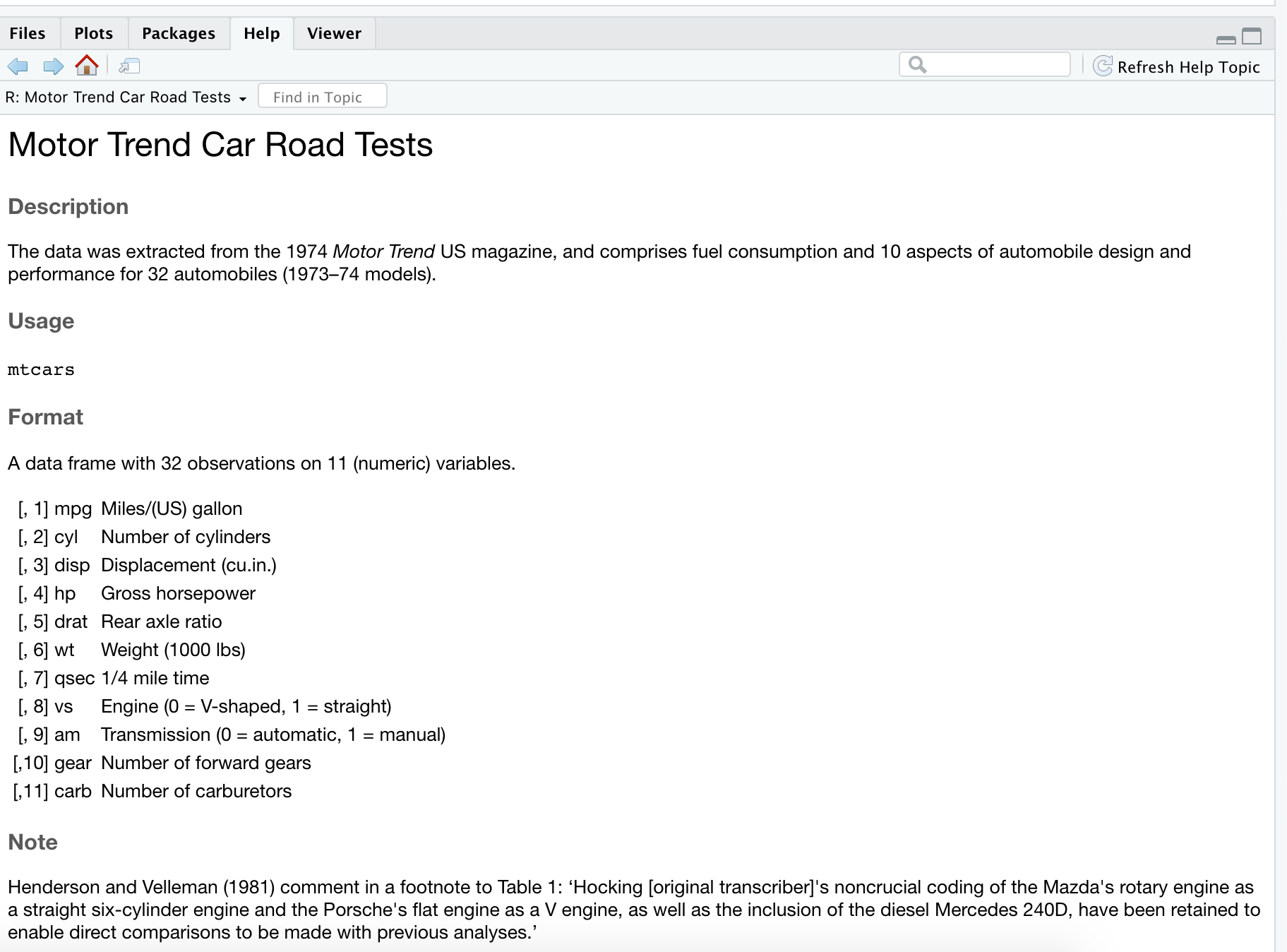 ] --- ## Descriptive Statistics - Data visualization: Graphics - Numerical measures - We are using R software for data analysis and modeling --- # What is R? - R is a software environment for statistical computing and graphics - Language designers: **R**oss Ihaka and **R**obert Gentleman at the University of Auckland, New Zealand - Parent language: S - The latest R version 3.6.2 has been released on 2019-12-12 --- # Why R? - **Free** - **Powerful:** Over 18000 contributed packages on the main repository (CRAN), as of July 2022, provided by top international researchers and programmers - **Flexible:** It is a language, and thus allows you to create your own solutions - **Community:** Large global community friendly and helpful, lots of resources --- Numerical summary measures ```r summary(mtcars) ``` ``` ## mpg cyl disp hp ## Min. :10.40 Min. :4.000 Min. : 71.1 Min. : 52.0 ## 1st Qu.:15.43 1st Qu.:4.000 1st Qu.:120.8 1st Qu.: 96.5 ## Median :19.20 Median :6.000 Median :196.3 Median :123.0 ## Mean :20.09 Mean :6.188 Mean :230.7 Mean :146.7 ## 3rd Qu.:22.80 3rd Qu.:8.000 3rd Qu.:326.0 3rd Qu.:180.0 ## Max. :33.90 Max. :8.000 Max. :472.0 Max. :335.0 ## drat wt qsec vs ## Min. :2.760 Min. :1.513 Min. :14.50 Min. :0.0000 ## 1st Qu.:3.080 1st Qu.:2.581 1st Qu.:16.89 1st Qu.:0.0000 ## Median :3.695 Median :3.325 Median :17.71 Median :0.0000 ## Mean :3.597 Mean :3.217 Mean :17.85 Mean :0.4375 ## 3rd Qu.:3.920 3rd Qu.:3.610 3rd Qu.:18.90 3rd Qu.:1.0000 ## Max. :4.930 Max. :5.424 Max. :22.90 Max. :1.0000 ## am gear carb ## Min. :0.0000 Min. :3.000 Min. :1.000 ## 1st Qu.:0.0000 1st Qu.:3.000 1st Qu.:2.000 ## Median :0.0000 Median :4.000 Median :2.000 ## Mean :0.4062 Mean :3.688 Mean :2.812 ## 3rd Qu.:1.0000 3rd Qu.:4.000 3rd Qu.:4.000 ## Max. :1.0000 Max. :5.000 Max. :8.000 ``` --- Numerical summary measures (cont.) ``` ## mpg cyl disp hp ## Min. :10.40 Min. :4.000 Min. : 71.1 Min. : 52.0 ## 1st Qu.:15.43 1st Qu.:4.000 1st Qu.:120.8 1st Qu.: 96.5 ## Median :19.20 Median :6.000 Median :196.3 Median :123.0 ## Mean :20.09 Mean :6.188 Mean :230.7 Mean :146.7 ## 3rd Qu.:22.80 3rd Qu.:8.000 3rd Qu.:326.0 3rd Qu.:180.0 ## Max. :33.90 Max. :8.000 Max. :472.0 Max. :335.0 ## drat wt qsec vs ## Min. :2.760 Min. :1.513 Min. :14.50 Min. :0.0000 ## 1st Qu.:3.080 1st Qu.:2.581 1st Qu.:16.89 1st Qu.:0.0000 ## Median :3.695 Median :3.325 Median :17.71 Median :0.0000 ## Mean :3.597 Mean :3.217 Mean :17.85 Mean :0.4375 ## 3rd Qu.:3.920 3rd Qu.:3.610 3rd Qu.:18.90 3rd Qu.:1.0000 ## Max. :4.930 Max. :5.424 Max. :22.90 Max. :1.0000 ## am gear carb ## Min. :0.0000 Min. :3.000 Min. :1.000 ## 1st Qu.:0.0000 1st Qu.:3.000 1st Qu.:2.000 ## Median :0.0000 Median :4.000 Median :2.000 ## Mean :0.4062 Mean :3.688 Mean :2.812 ## 3rd Qu.:1.0000 3rd Qu.:4.000 3rd Qu.:4.000 ## Max. :1.0000 Max. :5.000 Max. :8.000 ``` --- .pull-left[ ### Measures of central tendancy - Mean - Median - Mode ] .pull-right[ ### Measures of dispersion - Range - Inter quartile range - Variance - Standard deviation ] --- background-image: url('renv.png') background-position: center background-size: contain ## R environment --- background-image: url('rstudio1.png') background-position: center background-size: contain ## The RStudio IDE --- background-image: url('rstudio2.png') background-position: center background-size: contain ## The RStudio IDE .footer-note[.tiny[.green[Image Credit: ][Clastic Detritus ](https://clasticdetritus.com/2013/01/10/creating-data-plots-with-r/)]] --- background-image: url('airport.jpg') background-position: center background-size: cover .content-box-yellow[ ## R and RStudio ] .footer-note[.tiny[.green[Image Credit: ][Clastic Detritus ](https://clasticdetritus.com/2013/01/10/creating-data-plots-with-r/)]] --- background-image: url('airport.jpg') background-position: center background-size: cover .content-box-yellow[ ## R and RStudio ] .footer-note[.tiny[.green[Image Credit: ][Clastic Detritus ](https://clasticdetritus.com/2013/01/10/creating-data-plots-with-r/)]] --- "If R were **an airplane**, RStudio would be **the airport**, providing many, many supporting services that make it easier for you, the pilot, to take off and go to awesome places. Sure, you can fly an airplane without an airport, but having those runways and supporting infrastructure is a game-changer." -- Julie Lowndes --- class: inverse, center, middle # Create a new project --- background-image: url('project1.png') background-position: center background-size: contain --- background-image: url('project2.png') background-position: center background-size: contain --- background-image: url('project3.png') background-position: center background-size: contain --- background-image: url('project4.png') background-position: center background-size: contain --- background-image: url('project5.png') background-position: center background-size: contain --- background-image: url('project6.png') background-position: center background-size: contain --- ## R Console ```r 7+1 ``` ``` [1] 8 ``` ```r rnorm(10) ``` ``` [1] -0.572542604 -1.363291256 -0.388722244 0.277914132 -0.823081122 [6] -0.068840934 -1.167662326 -0.008309014 0.128855402 -0.145875628 ``` --- ## Variable assignment ```r a <- rnorm(10) a ``` ``` [1] -0.16391096 1.76355200 0.76258651 1.11143108 -0.92320695 0.16434184 [7] 1.15482519 -0.05652142 -2.12936065 0.34484576 ``` -- ```r b <- a*100 b ``` ``` [1] -16.391096 176.355200 76.258651 111.143108 -92.320695 16.434184 [7] 115.482519 -5.652142 -212.936065 34.484576 ``` --- # Data permanency - `ls()` can be used to display the names of the objects which are currently stored within R. - The collection of objects currently stored is called the **workspace** ```r ls() ``` ``` [1] "a" "A" "a1" "a2" "b" "B" "b1" "b2" [9] "b3" "C" "c1" "c2" "df" "g1" "Gender" "ID" [17] "mtcars" "p1" "w1" "w2" "w3" "Weight" ``` --- - To remove objects the function `rm` is available - remove all objects `rm(list=ls())` - remove specific objects `rm(x, y, z)` ```r rm(a) ls() ``` ``` [1] "A" "a1" "a2" "b" "B" "b1" "b2" "b3" [9] "C" "c1" "c2" "df" "g1" "Gender" "ID" "mtcars" [17] "p1" "w1" "w2" "w3" "Weight" ``` ```r rm(list=ls()) ls() ``` ``` character(0) ``` --- background-image: url('project7.png') background-position: center background-size: contain -- .pull-left[.full-width[.content-box-yellow[**At the end of an R session, if save: the objects are written to a file called .RData in the current directory, and the command lines used in the session are saved to a file called .Rhistory**]]] --- background-image: url('p81.png') background-position: center background-size: cover .pull-left[.full-width[.content-box-yellow[When R is started at later time **from the same directory** ]]] --- background-image: url('p82.png') background-position: center background-size: cover .pull-left[.full-width[.content-box-yellow[When R is started at later time **from the same directory** it reloads the **associated workspace** and **commands history.**]]] --- background-image: url('project9.png') background-position: center background-size: cover -- .pull-left[.full-width[.content-box-yellow[When R is started at later time **from the same directory** it reloads the **associated workspace** and **commands history.**]]] --- ## Comment your code - Each line of a comment should begin with the comment symbol and a single space: # . ```r rnorm(10) # This is a comment ``` ``` [1] -1.9049554 -0.8111702 1.3240043 0.6156368 1.0916690 0.3066049 [7] -0.1101588 -0.9243128 1.5929138 0.0450106 ``` ```r sum(1:10) # 1+2 ``` ``` [1] 55 ``` --- ## Style Guide - Good coding style is like correct punctuation: you can manage without it, butitsuremakesthingseasiertoread. -- Hadley Wickham ```r sum(1:10)#Bad commenting style ``` ``` [1] 55 ``` ```r sum(1:10) # Good commenting style ``` ``` [1] 55 ``` - Also, use commented lines of - and = to break up your file into easily readable sub-sections. ```r # Read data ---------------- # Plot data ---------------- ``` To learn more read Hadley Wickham's [Style guide](http://adv-r.had.co.nz/Style.html). --- ## Objects in R - R is an [object-oriented language](https://en.wikipedia.org/wiki/Object-oriented_programming). -- - An object in R is anything (data structures, functions, etc., that can be assigned to a variable). --- Let's take a look of some common types of objects. -- **1. Data structures** are the ways of arranging data. - You can create objects, using the left pointing arrow <- --- **2. Functions** tell R to do something. - A function may be applied to an object. - Result of applying a function is usually an object too. - All function calls need to be followed by parentheses. --- ## Example ```r a <- 1:20 # data structure sum(a) # sum is a function applied on a ``` ``` [1] 210 ``` ```r help.start() # Some functions work on their own. ``` --- # Getting help with functions and features - R has inbuilt help facility ### Method 1 ```r help(rnorm) ``` - For a feature specified by special characters such as `for`, `if`, `[[` ```r help("[[") ``` --- - Search the help files for a word or phrase. ```r help.search(‘weighted mean’) ``` ### Method 2 ```r ?rnorm ``` ```r ??rnorm ``` --- background-image: url('dataStructures.png') background-position: center background-size: contain ## Data structures .footer-note[.tiny[.green[Image Credit: ][venus.ifca.unican.es](http://venus.ifca.unican.es/Rintro/dataStruct.html)]] --- ## Data structures Data structures differ in terms of, - Type of data they can hold - How they are created - Structural complexity - Syntax to identify and access individual elements --- class: duke-green, center, middle # 1. Vectors --- # Vectors - Vectors are one-dimensional arrays that can hold numeric data, character data, or logical data. - Combine function c() is used to form the vector. - Data in a vector must only be one type or mode (numeric, character, or logical). You can’t mix modes in the same vector. --- ## Vector assignment **Syntax** ```r vector_name <- c(element1, element2, element3) ``` ```r x <- c(5, 6, 3, 1 , 100) ``` - assignment operator ('<-'), '=' can be used as an alternative. - `c()` function --- .red[What will be the output of the following code?] ```r y <- c(x, 500, 600) ``` --- # Types and tests with vectors ```r first_vec <- c(10, 20, 50, 70) second_vec <- c("Jan", "Feb", "March", "April") third_vec <- c(TRUE, FALSE, TRUE, TRUE) fourth_vec <- c(10L, 20L, 50L, 70L) ``` To check if it is a - vector: `is.vector()` ```r is.vector(first_vec) ``` ``` [1] TRUE ``` --- - charactor vector: `is.charactor()` ```r is.character(first_vec) ``` ``` [1] FALSE ``` - double: `is.double()` ```r is.double(first_vec) ``` ``` [1] TRUE ``` --- - integer: `is.integer()` ```r is.integer(first_vec) ``` ``` [1] FALSE ``` -- - logical: `is.logical()` ```r is.logical(first_vec) ``` ``` [1] FALSE ``` --- - length ```r length(first_vec) ``` ``` [1] 4 ``` --- # Coercion Vectors must be homogeneous. When you attempt to combine different types they will be coerced to the most flexible type so that every element in the vector is of the same type. Order from least to most flexible `logical` --> `integer` --> `double` --> `character` --- ```r a <- c(3.1, 2L, 3, 4, "GPA") typeof(a) ``` ``` [1] "character" ``` ```r anew <- c(3.1, 2L, 3, 4) typeof(anew) ``` ``` [1] "double" ``` --- ### Explicit coercion Vectors can be explicitly coerced from one class to another using the `as.*` functions, if available. For example, `as.charactor`, `as.numeric`, `as.integer`, and `as.logical`. --- ```r vec1 <- c(TRUE, FALSE, TRUE, TRUE) typeof(vec1) ``` ``` [1] "logical" ``` ```r vec2 <- as.integer(vec1) typeof(vec2) ``` ``` [1] "integer" ``` ```r vec2 ``` ``` [1] 1 0 1 1 ``` --- .red[Why does the below output NAs?] ```r x <- c("a", "b", "c") as.numeric(x) ``` ``` [1] NA NA NA ``` --- .pull-left[ ```r x1 <- 1:3 x2 <- c(10, 20, 30) combinedx1x2 <- c(x1, x2) combinedx1x2 ``` ``` [1] 1 2 3 10 20 30 ``` ] -- .pull-right[ ```r class(x1) ``` ``` [1] "integer" ``` ```r class(x2) ``` ``` [1] "numeric" ``` ```r class(combinedx1x2) ``` ``` [1] "numeric" ``` ] --- - If you combine a numeric vector and a character vector ```r y1 <- c(1, 2, 3) y2 <- c("a", "b", "c") c(y1, y2) ``` ``` [1] "1" "2" "3" "a" "b" "c" ``` --- # Name elements in a vector You can name elements in a vector in different ways. We will learn two of them. When creating it ```r x1 <- c(a=1991, b=1992, c=1993) x1 ``` ``` ## a b c ## 1991 1992 1993 ``` --- Modifying the names of an existing vector ```r x2 <- c(1, 5, 10) names(x2) <- c("a", "b", "b") x2 ``` ``` ## a b b ## 1 5 10 ``` Note that the names do not have to be unique. --- # To remove names of a vector Method 1 ```r unname(x1); x1 ``` ``` [1] 1991 1992 1993 ``` ``` a b c 1991 1992 1993 ``` --- Method 2 ```r names(x2) <- NULL; x2 ``` ``` [1] 1 5 10 ``` What will be the output of the following code? ```r v <- c(1, 2, 3) names(v) <- c("a") v ``` --- ### Simplifying vector creation - colon `:` produce regular spaced ascending or descending sequences. ```r 10:16 ``` ``` [1] 10 11 12 13 14 15 16 ``` ```r -0.5:8.5 ``` ``` [1] -0.5 0.5 1.5 2.5 3.5 4.5 5.5 6.5 7.5 8.5 ``` --- - sequence: `seq(initial_value, final_value, increment)` ```r seq(1,11) ``` ``` [1] 1 2 3 4 5 6 7 8 9 10 11 ``` ```r seq(1, 11, length.out=5) ``` ``` [1] 1.0 3.5 6.0 8.5 11.0 ``` ```r seq(0, 11, by=2) ``` ``` [1] 0 2 4 6 8 10 ``` --- - repeats `rep()` ```r rep(9, 5) ``` ``` [1] 9 9 9 9 9 ``` ```r rep(1:4, 2) ``` ``` [1] 1 2 3 4 1 2 3 4 ``` ```r rep(1:4, each=2) # each element is repeated twice ``` ``` [1] 1 1 2 2 3 3 4 4 ``` --- ```r rep(1:4, times=2) # whole sequence is repeated twice ``` ``` [1] 1 2 3 4 1 2 3 4 ``` ```r rep(1:4, each=2, times=3) ``` ``` [1] 1 1 2 2 3 3 4 4 1 1 2 2 3 3 4 4 1 1 2 2 3 3 4 4 ``` ```r rep(1:4, 1:4) ``` ``` [1] 1 2 2 3 3 3 4 4 4 4 ``` ```r rep(1:4, c(4, 1, 4, 2)) ``` ``` [1] 1 1 1 1 2 3 3 3 3 4 4 ``` --- ## Logical operators ```r c(1, 2, 3) == c(10, 20, 3) ``` ``` [1] FALSE FALSE TRUE ``` ```r c(1, 2, 3) != c(10, 20, 3) ``` ``` [1] TRUE TRUE FALSE ``` ```r 1:5 > 3 ``` ``` [1] FALSE FALSE FALSE TRUE TRUE ``` --- ```r 1:5 < 3 ``` ``` [1] TRUE TRUE FALSE FALSE FALSE ``` - `<=` less than or equal to - `>=` greater than or equal to - `|` or - `&` and --- # Operators: `%in%` - in the set ```r a <- c(1, 2, 3) b <- c(1, 10, 3) a%in%b ``` ``` [1] TRUE FALSE TRUE ``` ```r x <- 1:10 y <- 1:3 ``` --- ```r x ``` ``` [1] 1 2 3 4 5 6 7 8 9 10 ``` ```r y ``` ``` [1] 1 2 3 ``` ```r x %in% y ``` ``` [1] TRUE TRUE TRUE FALSE FALSE FALSE FALSE FALSE FALSE FALSE ``` ```r y %in% x ``` ``` [1] TRUE TRUE TRUE ``` --- ## Vector arithmetic - operations are perfored element by element. ```r c(10, 100, 100) + 2 # two is added to every element in the vector ``` ``` [1] 12 102 102 ``` -- - operations between two vectors ```r v1 <- c(1, 2, 3); v2 <- c(10, 100, 1000) v1 + v2 ``` ``` [1] 11 102 1003 ``` --- Add two vectors of unequal length ```r longvec <- seq(10, 100, length=10); shortvec <- c(1, 2, 3, 4, 5) shortvec + longvec ``` ``` [1] 11 22 33 44 55 61 72 83 94 105 ``` .red[What will be the output of the following code?] ```r first <- c(1, 2, 3, 4); second <- c(10, 100) first * second ``` --- ## References Le Dinh, T., Lee, S. H., Kwon, S. G., & Kwon, K. R. (2022). COVID-19 Chest X-ray Classification and Severity Assessment Using Convolutional and Transformer Neural Networks. Applied Sciences, 12(10), 4861.